
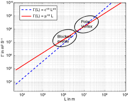
Fig. 1
The order of magnitude of circulations with respect to different lengths scales for the dissipation of energy ɛ=5·10−4 m2 s−3 and the dissipation of circulation µ=264 m2 s−2 .
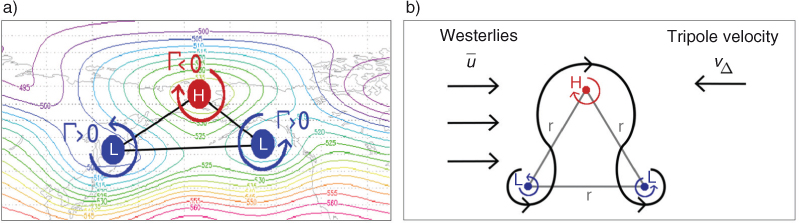
Fig. 2
(a) A three-point vortex equilibrium describes an omega block (geopotential mean over the North Pacific 1–12 March 2011). (b) Such a three-vortex system that represents an omega block translates eastwards, if the total circulation Γ=Γ1+Γ2+Γ3 vanishes. Stationarity can be explained if the translation velocity v Δ westwards is equal to the velocity of the zonal mean flow eastwards denoted as westerlies in the meteorological context.
Table 1. Initial and final (averaged) configurations of the trapezoids for the omega blocks over Russia in summer 2010 and over the North Pacific in March 2011
Points of initial trapezoid(10 ° E, 80 ° N) (80 ° E, 80 ° N)(160 ° E, 85 ° N) (220 ° E, 85 ° N)(10 ° W, 35 ° N) (100 ° E, 35 ° N)(140 ° E, 45 ° N) (240 ° E, 45 ° N)Adjustment of northern line80 ° N → 70 ° N by 2.5 °85 ° N → 75 ° N by 2.5 °Adjustment of southern basis25 ° N → 45 ° N by 2.5 °35 ° N → 55 ° N by 2.5 °Final averaged height32.5 ° N–75 ° N46.9 ° N–80 ° N

Fig. 3
Trapezoid approximating the region of the omega block. In the green area, the total cyclonic circulation is calculated, and in the yellow area, the total cyclonic circulation is determined. The total anticyclonic circulation ΓHigh is calculated in the striped area.
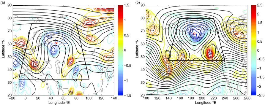
Fig. 4
Temporal averages [(a) 24 July 2010, 00 UTC to 7 August 2010, 18 UTC and (b) 1 March 2011, 00 UTC to 11 March 2011, 12 UTC] of geopotential height (black contours) and relative vorticity (in 10−5 s−1, coloured contours). The vorticity is shown in the field of kinematic vorticity number W k >1. The trapezoids encircle the area of zero total circulation, and the blue and red circles mark centres of the low- and high-pressure areas, respectively. Note the different ranges of vorticity in the plots.
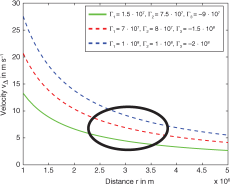
Fig. 5
Translational velocity of a three-point vortex system as a function of the intervortical distances r for three different vortex configurations with vanishing total circulation is shown. For typical distances on a synoptic scale of 2500–3500 km, the absolute value of the analytical translation velocity of 5–10 ms−1 of a three-point vortex equilibrium coincides with the typical basic flow velocity.
Table 2. Values of the circulation of the tripole and the locations of the centres over Russia and Europe in summer 2010 and over the North Pacific in March 2011
Circulation in m2 s−1Location (°N; °E)Circulation in m2 s−1Location (°N; °E)
ΓLow17.543.107(45.8; 17.7)7.090.107(51.7; 166.7)ΓLow25.424.107(45.1; 70.9)8.322.107(53.0; 214.3)ΓHigh1−1.306.108(60.7; 48.9)−1.546.108(67.8; 186.0)

Fig. 6
(a) The equilibrium state for the initial states and Γ1=1, Γ2=−2, Γ3=1, which builds an equilateral triangle where total sum of circulations equals zero. (b) Small perturbations of x3 lead to cycloid motions.

Fig. 7
The quasi-biennial oscillation. The dashed line represents the mean vorticity, and the solid line represents the zonal wind. The data is averaged over 0–20 ° N in 30 hPa.
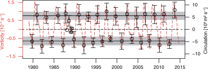
Fig. 8
The dashed line presents the vorticity, averaged over 0–20 ° N. The circles indicate the calculated circulation during a single QBO phase (defined by the sign of the vorticity) and the corresponding bars the first standard deviation. The two solid, horizontal lines are the resulting mean circulation for the West and East phase of the QBO respectively. Their standard deviation is marked by the grey-shaded area. The used circulation , displayed by the two dotted lines, lies within the first standard deviation.
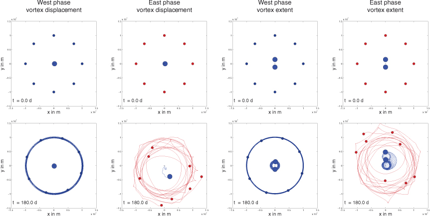
Fig. 9
The perturbed initial states (first row) and the resulting trajectories (second row) are shown for the QBO west phase with cyclonic, outer point vortices (first and third column, coloured blue) and the QBO east phase with anticyclonic, outer point vortices (second and forth column, coloured red). The first and second columns contain the displacement of the central vortex and the third and fourth columns the additional point vortex.
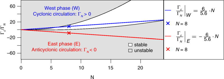
Fig. 10
Stability diagram based on the stability criterion of Cabral and Schmidt (2000) given in eq. (26). The two lines represent the approximate scale of the stratospheric circulations. The vortex states for the west phase (blue line) are stable in a large range, whereas no stable configurations can be found for the east phase (red line). Here, Γ N =ΓQBO N −1 denotes the circulation of each outer vortex with ΓQBO=5.6·108 m2 s−1, and Γ c =6·108 m2 s−1 represents the polar vortex.