
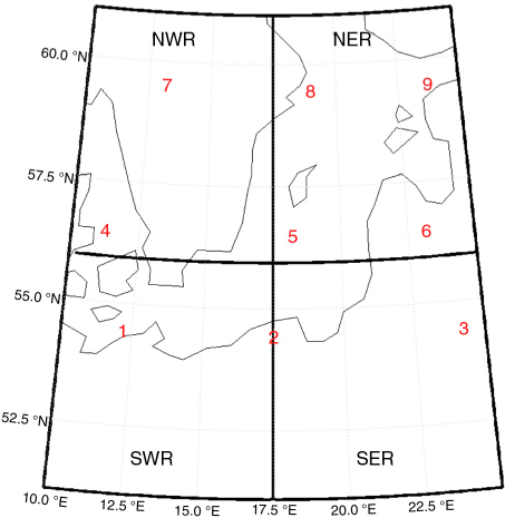
Fig. 1
Area of study showing nine points which are used to illustrate the geographical subdivisions. The black lines demonstrate the area subdivisions (SWR, SER, NWR, NER) used in Section 4.2.
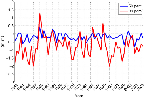
Fig. 2
Difference of the 50th percentiles (blue) and 98th percentiles (red) of wind speed between coastDat2 and HiResAFF data sets during winter (DJF). The figure displays the mean over the area shown in Fig. 1.
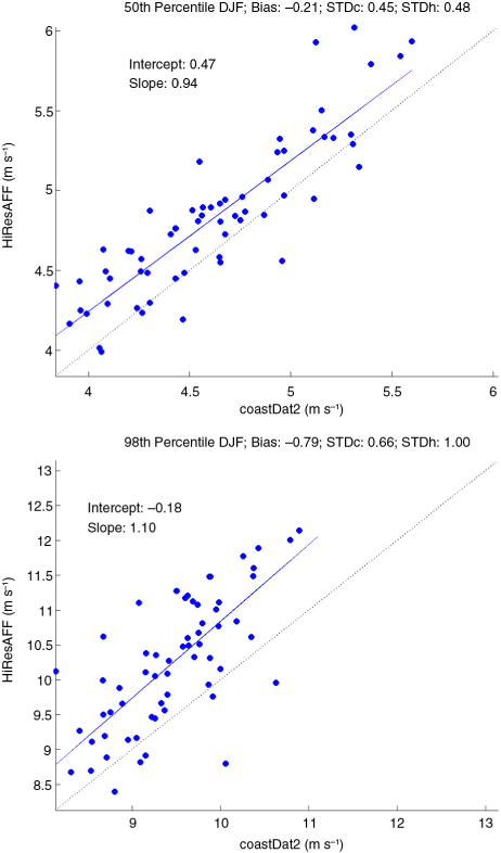
Fig. 3
Scatter plot of the 50th (upper) and 98th (lower) percentiles of wind speed of each winter for coastDat2 and HiResAFF for the period 1948–2009. The blue line represents the linear regression and the light grey line the one-to-one-correspondence line. The figure shows the mean over the area displayed in Fig. 1. STD - standard deviation; c - coastDat2; h – HiResAFF.
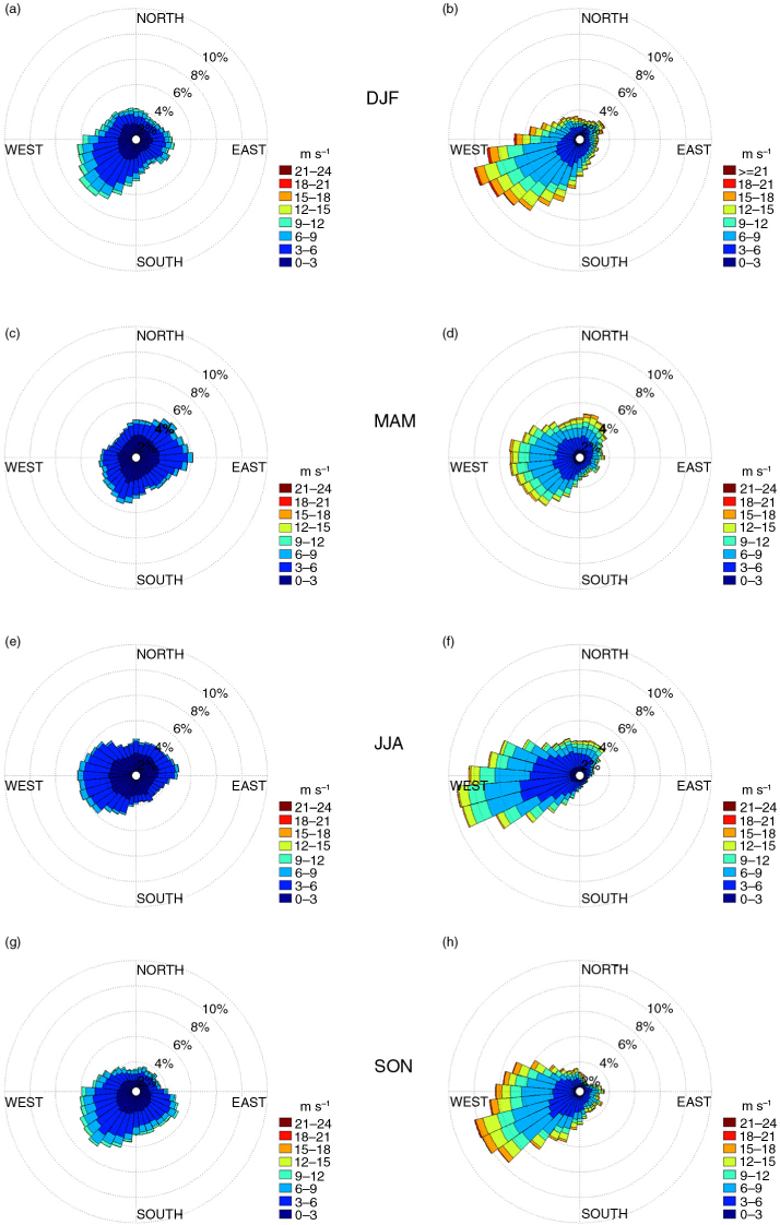
Fig. 4
Wind roses of median (left: a, c, e, g) and extreme (right: b, d, f, h) wind in coastDat2 (1948–2009). The colours show the intensity (in m s−1) and the bins show the direction from which the wind blows. Median events are defined as the three wind events per season which are closest to the 50th percentile of wind speed. Extremes are determined as the three strongest wind events per season.
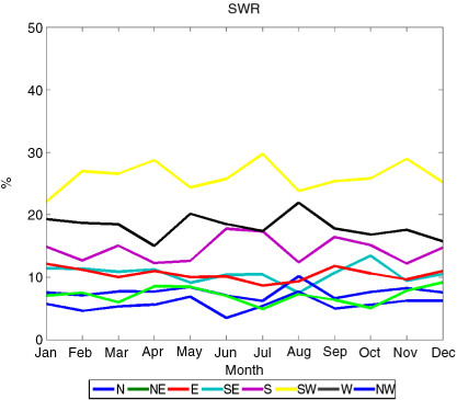
Fig. 5
Annual cycle of the eight main wind directions of coastDat2 (1948–2009) for the south-western Baltic Sea region (SWR in Fig. 1). This figure only includes the three wind events per month with intensities closest to the 50th percentile of wind speed per month. Units are monthly mean frequency in %.
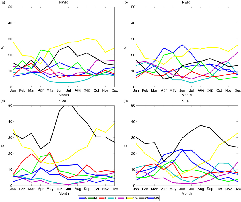
Fig. 6
Annual cycle of the eight main wind directions for extreme events of coastDat2 (1948–2009) in (a) north-western (NWR), (b) north-eastern (NER), (c) south-western (SWR) and (d) south-eastern (SER) Baltic Sea (see Fig. 1). Extremes are defined by the 90th percentile of wind speed per month. Units are monthly mean frequency in %.
Table 1. Explained variance in % of the three leading EOF patterns for each season derived from HiResAFF (1850–2009 and 1948–2009) and coastDat2 (1948–2009). Results for monthly mean wind are shown as plain text and results for wind events exceeding the 98th percentile in bold
DJF65, 4125, 316, 1196, 82 MAM58, 3828, 327, 1293, 82 JJA50, 4830, 299, 889, 86 SON54, 4633, 277, 1195, 84HiResAFF (1948–2009) DJF64, 4625, 256, 1196, 82 MAM59, 4529, 316, 893, 84 JJA50, 3929, 3310, 1189, 83 SON61, 4327, 287, 1195, 82coastDat2 (1948–2009) DJF63, 3922, 358, 993, 83 MAM56, 4324, 298, 1188, 83 JJA56, 4718, 2513, 1187, 83 SON55, 3927, 369, 1491, 89
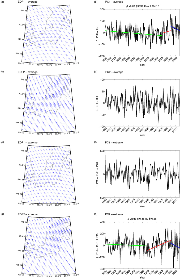
Fig. 7
First leading EOF patterns together with their PC time series for average wind [upper four panels: (a–d)] and extreme wind [lower four panels: (e–h)] events of the HiResAFF data set (1850–2009). The left-hand side panels show the pattern of variability of the combined u and v EOF analysis (see Section 2.4). Arrows are not scaled for the sake of clarity. The right-hand side panels show the corresponding principal component time series. The coloured lines in (b) and (h) show trends on different time scales. The significance values (p-values) for the green (g), red (r) and blue (b) lines are shown above the figures. Explained variances are indicated in Table 1.