
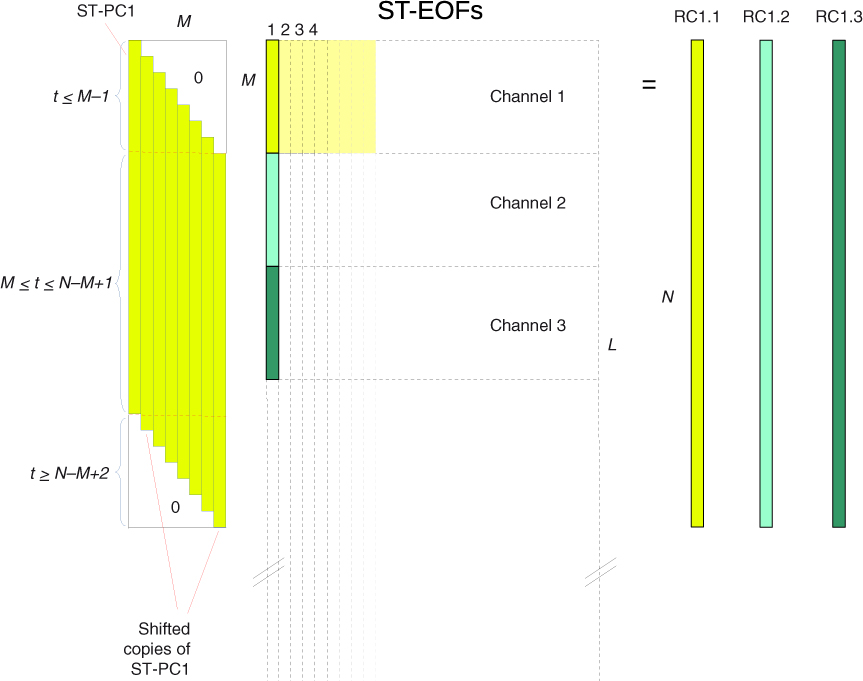
Fig. 1
Example calculation of the reconstructed components (RCs). A matrix of M shifted copies of a ST-PC (ST-PC1 in this example) is constructed to calculate reconstructions of that ST-PC in a time series of each channel (grid point). This matrix is then multiplied with that part of ST-EOF that corresponds to each channel. If t≤M, the elements of RC are divided by t, if M≤t≤N−M+1, divided by M, and if t≥N−M+2, divided by N−t+1.
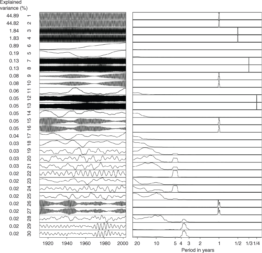
Fig. 2
ST-PCs 1–30 of 20CR monthly near-surface temperature 1901–2012 and their spectra. The lag window length M used in RMSSA is 20 yr (240 months). The data set is centred and algorithm 1 of Appendix A.2 is applied. The proportion of the variance explained by each component is also presented in the figure.
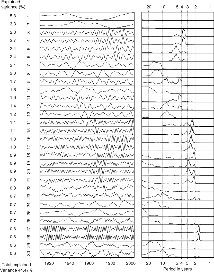
Fig. 3
ST-PCs 1–30 of 20CR monthly near-surface temperature 1901–2012 and their spectra. The lag window length M used in RMSSA is 20 yr (240 months). The annual cycle and linear trend are removed from the original data set and algorithm 2 of Appendix A.2 is applied. The proportion of the remaining variance explained by each component is also presented in the figure.
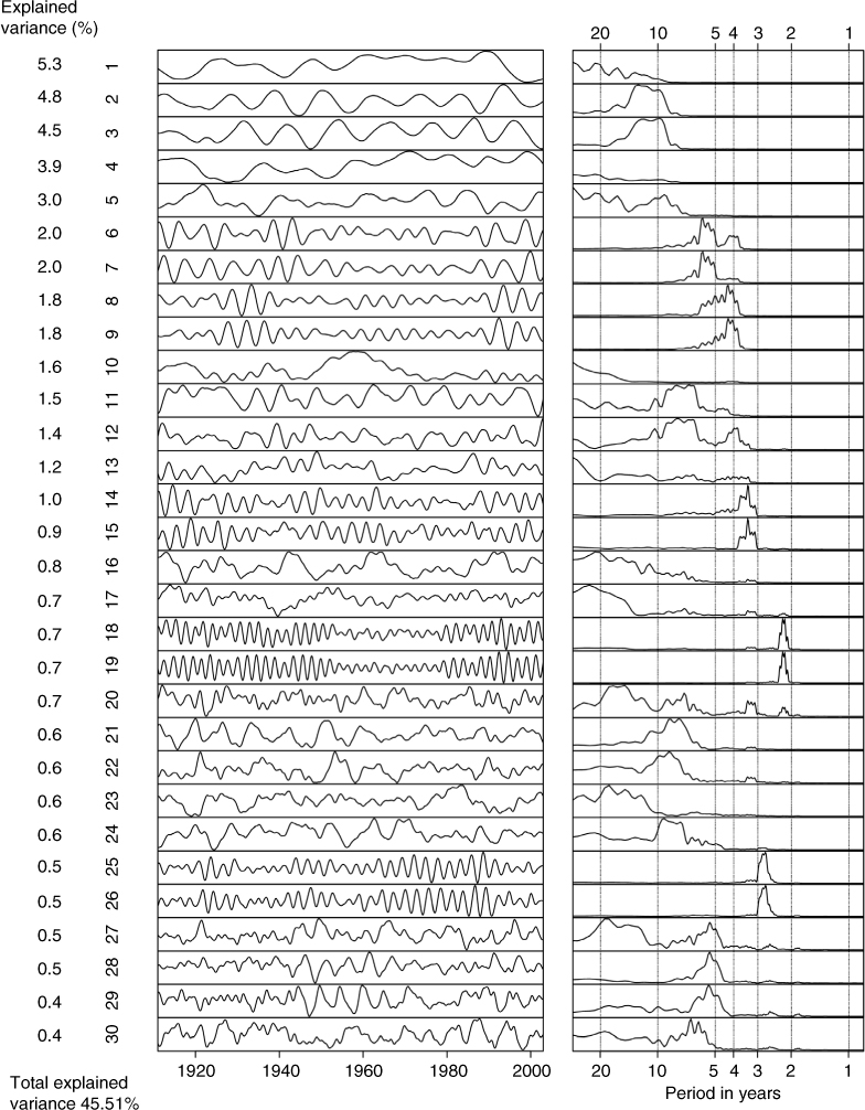
Fig. 4
ST-PCs 1–30 of HadGEM2 monthly near-surface temperature 1901–2012 and their spectra. The lag window length M used in RMSSA is 20 yr (240 months). The annual cycle and linear trend are removed from the original data set and algorithm 2 of Appendix A.2 is applied. The proportion of the remaining variance explained by each component is also presented in the figure.
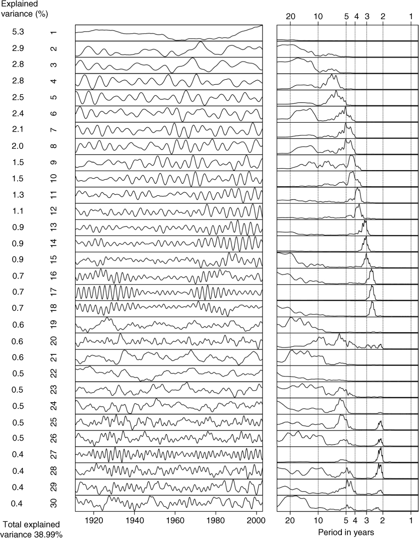
Fig. 5
ST-PCs 1–30 of MPI-ESM monthly near-surface temperature 1901–2012 and their spectra. The lag window length M used in RMSSA is 20 yr (240 months). The annual cycle and linear trend are removed from the original data set and algorithm 2 of Appendix A.2 is applied. The proportion of the remaining variance explained by each component is also presented in the figure.
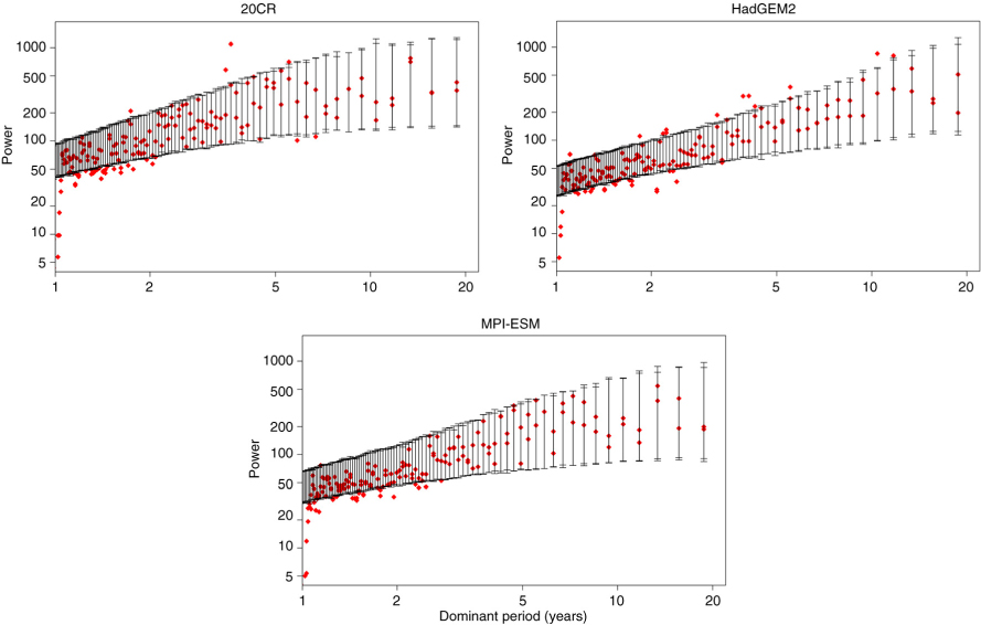
Fig. 6
MC-MSSA test of the monthly near-surface temperature variability in 20CR, HadGEM2 and MPI-ESM data sets 1901–2012. PCs 1–30 of RP + PCA (see Appendix A.2, algorithm 2) are used as input channels in the analysis and the lag window length M is 20 yr (240 months). In MC-MSSA, the red-noise basis is used. Red squares show the data eigenvalues plotted against the dominant frequency of the ST-PC corresponding to each eigenvalue. The vertical bars show the 2.5th and 97.5th percentiles of the eigenvalue distribution calculated from 1000 realisations of the red-noise surrogates. The ST-PCs that correspond to eigenvalues rising above the 97.5th percentiles are considered significant at the 5% level. Note the missing power at 1 yr due to the removal of the annual cycle.
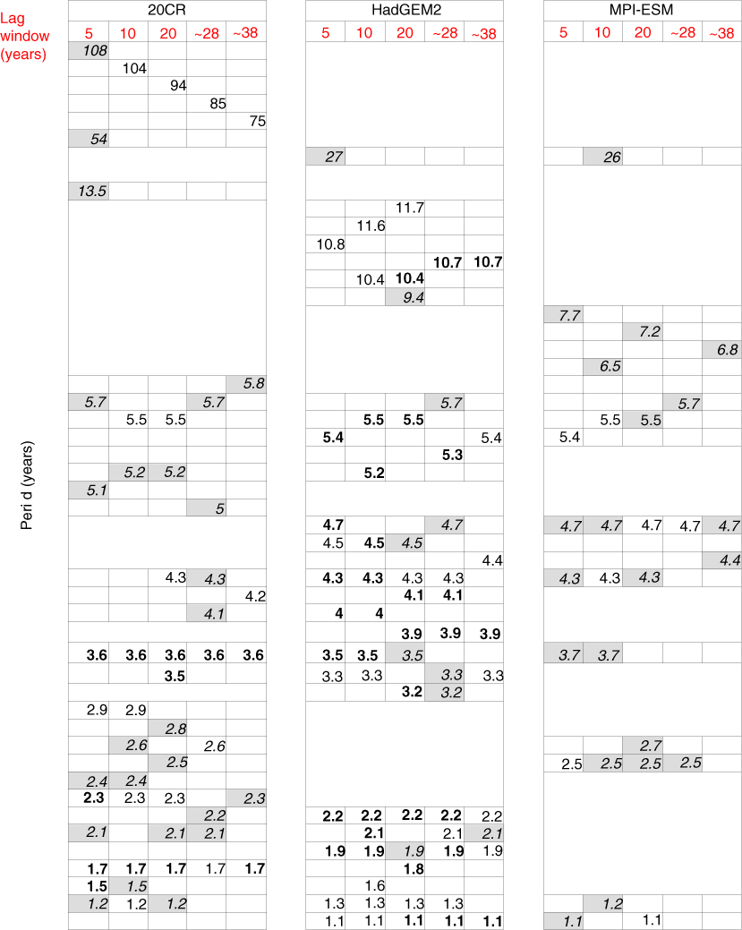
Fig. 7
Periodicities (years) detected by RMSSA/MC-MSSA with varying lag window length (years) for each data set (20CR, HadGEM2 and MPI-ESM). The similar periodicities among the data sets are aligned. Numbers in the figure are in bold if the significance level of a periodicity is 1%, and with grey background if 10%. Otherwise the significance level is 5%. Dominant frequencies of the oscillations are estimated using fast Fourier transform (FFT).
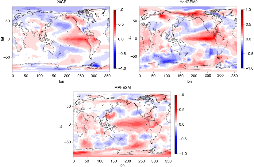
Fig. 8
Global patterns of ~5.5 yr oscillation of the near-surface temperature anomaly (°C) in 20CR, HadGEM2 and MPI-ESM data sets 1901–2012. The patterns are calculated as composites of eight cases, when the oscillation is in its maximum positive phase in the equatorial Pacific. Those positive events are defined as an average of winter months (Nov–Mar). See the text for more details on the reconstruction procedure. The identified patterns have similarities to El Niño -phenomenon.