A simple model of ocean temperature re-emergence and variability

2.1. Transition relations

Denote the years by a subscript i, and the summer and subsequent winter of year i by the subscripts Si and Wi, respectively. At the start of summer in year i, the initial temperature anomaly T _si0 is set equal to the anomaly T _Wi−1 at the end of the previous winter:

The temperature anomaly T _Wi0 at the start of winter in year i is found by instantaneously mixing the summer mixed layer and the sequestered winter layer heat content:

where T _Si denotes the end-of-summer temperature anomaly. Thus

where

is the ratio of the summer and winter mixed layer depths, with r≤1.

The term (1−r)T _Wi−1 contains the re-emergence mechanism, and to help monitor its effect in various circumstances we introduce a ‘process flag’ parameter γ in eq. (8), so

where 0≤γ≤1. Effectively the layer sequestered below the summer mixed layer emerges with a temperature anomaly reduced by the factor γ, and by setting γ=0 in later expressions the effect of re-emergence via persistence of anomalies in the sequestered layer can be removed.

Similarly, we introduce another process flag η in eq. (6) to monitor the contribution of preceding winter temperature anomalies that influence the following summer and winter by persisting in the summer mixed layer:

The season-to-season evolution is summarised in the schematic diagram in Fig. 1. Note that Schneider and Cornuelle (2005) introduced a similar two-season model that was integrated numerically to explore some re-emergence effects.

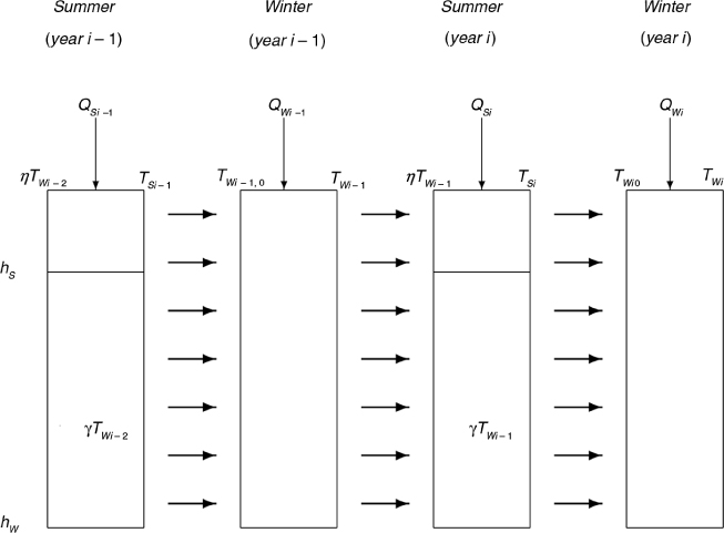
Fig. 1

2.2. Season-to-season relations

The duration of each season is $\mathrm{\Delta }t$=0.5 yr. Equation (2) can be integrated over this time interval, using the transition relation [eq. (11)], to relate the end-of-summer state to the end-of-previous-winter state:

where

measures the fraction by which temperature anomalies are attenuated through the summer season. Similarly, from eqs. (3) and (10),

where

Thus, using eq. (12), the relation between the end-of-winter state to the end-of-previous-winter state is

The interpretation of the terms appearing in eq. (12) is as follows:

• $f_S\eta T_{Wi-1}$ is the influence of preceding winter temperature anomalies on those at the end of summer.

• $(1-f_S)Q_{Si}/{\kappa }_S$ is the influence of the summer atmospheric forcing on the temperature at the end of summer.

The interpretation of the terms appearing in eq. (16) is as follows:

• $f_{W}r\eta f_S{T}_{Wi-1}$ represents the influence of preceding winter temperature anomalies that persist in the summer mixed layer, which survive after the entrainment process ends, on temperature anomalies at the end of the following winter.

• $f_W\gamma (1-r)T_{Wi-1}$ is the influence of re-emergence on temperature anomalies at the end of the following winter.

• $f_{W}r(1-f_S)Q_{Si}/{\kappa }_S$ measures the influence of the portion of the summer atmospheric forcing that survives after the entrainment process ends on temperature anomalies at the end of the following winter.

• $(1-f_W)Q_{Wi}/{\kappa }_W$ measures the influence of the winter atmospheric forcing on the temperature at the end of winter.

For simplicity the model is derived in terms of end-of-season values, but note that as the thermal forcing Q is constant within each season then the end-of-season temperature is also indicative of the season-average temperature and the model could be formulated in terms of seasonal averages.

Effectively the model is an auto-regressive system. For later reference, the winter-to-winter relation, eq. (16), is written as

where

with 0≤C≤1, and

is a net stochastic temperature contribution.

In particular, when η=γ=0 then C=0, the previous winter has no influence, and T _W evolution reduces to a white noise process.

Analytic expressions for the winter-to-winter and summer-to-winter correlations, the variance of the winter and summer temperature, and the power spectrum of the winter and summer temperature can be derived using eqs. (12) and (16), as described in the Appendix.

In exploring the effects of various parameters, departures from a set of standard values will be considered. Typical North Atlantic values of the damping parameters are κ _S =10Wm⁻²K⁻¹ and κ _W =25Wm⁻²K⁻¹ (e.g. Frankignoul et al., 1998; Deser et al., 2003). The summer mixed layer depth is fixed as h _S =25 m. The selected value for the standard deviation of the winter atmospheric forcing is ${\sigma }_{QW}=20\text{W}{\text{m}}^{-\text{2}}$, and for summer ${\sigma }_{QS}=10\text{W}{\text{m}}^{-\text{2}}$. For reference, model variables, parameters and standard values are summarised in Table 1.

The fraction f _S decreases as the damping κ _S increases. To quantify this effect, this dependence is shown in Fig. 2a: f _S is below 0.1 when κ _S is above about 15Wm⁻²K⁻¹. Likewise, as illustrated in Fig. 2b, f _W decreases as κ _W decreases, but increases as h _W increases.

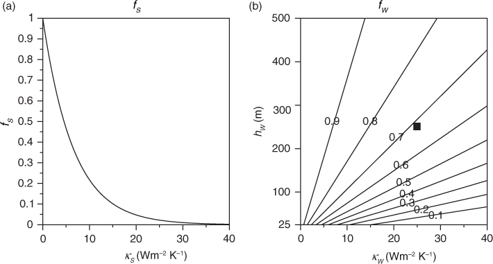
Fig. 2

3.1. The impact of varying κ _S and κ _W on Corr(T_W, T_W−1)

Figure 3a shows C with κ _W fixed and varying h _W and κ _S . (For reference, the black squares on this and subsequent diagrams indicate the standard values. Values of various statistics for standard values are provided in Table 2.) For large κ _S $f_S\ll 1$) the preceding winter anomalies that influence the summer layer have negligible influence through to winter, and C≈f_W (1−r). For small κ _S (f _S ≈1) the effect on C is weak. The winter depth h _W has a much larger influence on C: although C is less than 0.1 for h _W less than about 50 m, the correlation exceeds 0.5 for h _W greater than about 150 m when the re-emergence mechanism has a dominant influence.

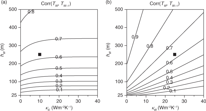
Fig. 3

In Fig. 3b κ _S is fixed while κ _W and h _W vary. Comparing the pattern of Fig. 3b with that of Fig. 2b, it is evident that C is strongly influenced by the attenuation factor f _W . Correlations are high for large h _W and small κ _W (e.g. larger than 0.8 when κ _W is less than about 10 Wm⁻²K⁻¹ and h _W larger than 250 m), when a relatively large heat content is sequestered for re-emergence.

It is interesting to compare the winter-to-winter correlation with the value when r=1. Let C ₁ denote the winter-to-winter correlation when r=1. From (20),

where f _W1 is the value of f _W when r=1. Then

where $\eta f_S(r{f}_W-f_{W1})$ represents the contribution of persistence via the summer mixed layer. When η=γ=1 it is straightforward to prove that C>C ₁ when h _W >h _S . Since f _W1<f _W for all h _W >h _S , and f _S <1,

which concludes the proof. The term rf _W appears often in the properties of the model, and for reference it is illustrated in Fig. 4 for a range of values of h _W and κ _W . As a function of h _W this term has a maximum at a depth $h_W=\mathrm{\Delta }t{\kappa }_W/{\rho }_0{c}_p$. When κ _W is less than about 7 Wm⁻²K⁻¹ that depth is less than h _S , and in Fig. 4 rf _W decreases as h _W increases. For larger κ _W , rf _W increases to a maximum and then decreases as h _W increases. The line with rf _W =f _W1 is also included in Fig. 4. Below this line persistence increases C−C ₁, but above the line persistence decreases C−C ₁.

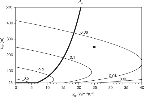
Fig. 4

This behaviour occurs due to the competing effects of h _W : increasing the winter mixed layer depth reduces the relative contribution of preceding winter temperature anomalies via persistence, but also reduces the rate at which they are damped through winter.

The relative effects of re-emergence and persistence on the winter-to-winter correlation as h _W varies can be compared. From eq. (20), with η=γ=1 , the former is larger than the latter when (1−r)>rf _S . This condition (which is independent of κ _W ) can be re-written as h _W >(1+f _S )h _S , and as 0<f _S <1, it follows that re-emergence always has the larger influence when h _W >2h _S .

To quantify the relative effects, the ratio rf _S /(1−r) is shown in Fig. 5 for varying h _W and κ _S . The ratio rapidly decreases as h _W increases, the more so as κ _S increases. For the standard value κ _S =10Wm⁻²K⁻¹ the ratio is 1 for h _W ≈30 m, but less than 0.2 when h _W >52 m. Unless the seasonal range of mixed layer depth is small, re-emergence has a much larger influence on the winter-to-winter persistence of temperature anomalies than that of preceding winter temperature anomalies that persist through the summer mixed layer.

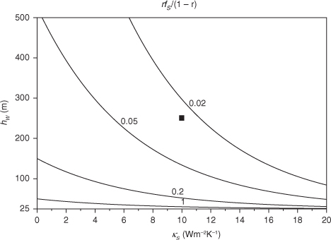
Fig. 5

4.1. The impact of varying κ _W and h_W on ${\sigma }_{TW}^2$

Figure 6 illustrates the effect of varying h _W and κ _W on the winter variance, with other parameters set to standard values. As shown in Fig. 6a, ${\sigma }_{TW}^2$ is largest when h _W =h _S and κ _W =0. (Note that as ${\kappa }_W\to 0$ then $(1-f_W)/{\kappa }_W\to \mathrm{\Delta }t/\rho c_p{h}_W$ and thus remains finite.) As expected, ${\sigma }_{TW}^2$ decreases as damping κ _W increases. For fixed κ _W , ${\sigma }_{TW}^2$ decreases as h _W increases, because the increased heat capacity of the deeper winter layer means less temperature change for the same heat input.

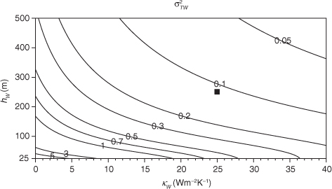
Fig. 6

The region with C=0.7 in Fig. 3b indicates approximately when the contribution to ${\sigma }_{TW}^2$ from ${\sigma }_P^2$ is greater than that of ${\sigma }_R^2$ (i.e. when C ²>0.5). For ${\kappa }_W\to 0$ this occurs when h _W is greater than about 70 m, and occurs at larger h _W as κ _W increases. For all κ _W , when h _W is very close to h _S , ${\sigma }_{TW}^2\approx {\sigma }_R^2$ and when h _W is close to 500 m, ${\sigma }_{TW}^2\approx {\sigma }_P^2$.

The winter and summer components ${\sigma }_{RS}^2$ and ${\sigma }_{RW}^2$ are plotted similarly in Fig. 7. (The ‘summer’ component depends on κ _W because the anomalies imposed in the summer season are attenuated through the following winter.) For the ranges of values shown ${\sigma }_{RW}^2$ (Fig. 7a) decreases as κ _W and h _W increase, and is much larger than ${\sigma }_{RS}^2$ (Fig. 7b). ${\sigma }_{RS}^2$ is negligible for all h _W because when h _W is close to h _S anomalies forced in the preceding summer are relatively strongly damped in a shallow winter mixed layer, whereas for larger h _W entrainment acts to significantly reduce their influence. Note that for κ _W above about 6 Wm⁻²K⁻¹, ${\sigma }_{RS}^2$ increases at first as h _W increases from h _S , then decreases: this is due to the effect of the factor rf _W as described in Section 3.1.

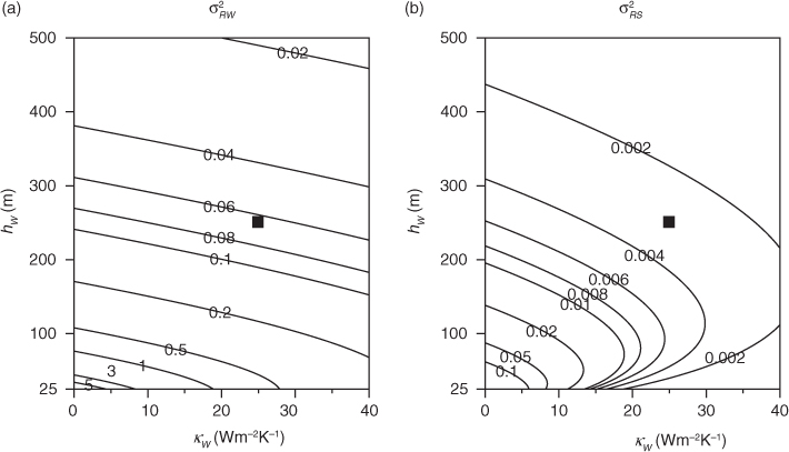
Fig. 7

The relative effects on σ _TW of the near-surface and sequestered pathways for winter-to-winter connections are explored by plotting ${\sigma }_P^2$ for γ=1, η=0 (Fig. 8a, sequestered path only) and for γ=0, η=1 (Fig. 8b, near-surface path only). Except for depths h _W close to h _S , the sequestered path has a much greater effect. Note that the behaviour of ${\sigma }_P^2$ with h _W when γ=0 and η=1 (Fig. 8b) is similar to that which was described for ${\sigma }_{RS}^2$, with the effect of the term rf _W again evident. It is also interesting to note that when γ=1, η=0, ${\sigma }_P^2$ increases as h _W increases from h _S , and then decreases. This is linked to the effects of decreasing the winter mixed layer depth on the effects of the atmospheric forcing and re-emergence: decreasing (increasing) the winter mixed layer increases (decreases) the size of the temperature anomalies via the atmospheric forcing, which acts to increase (decrease) the effects of re-emergence on the temperature in the following winter.

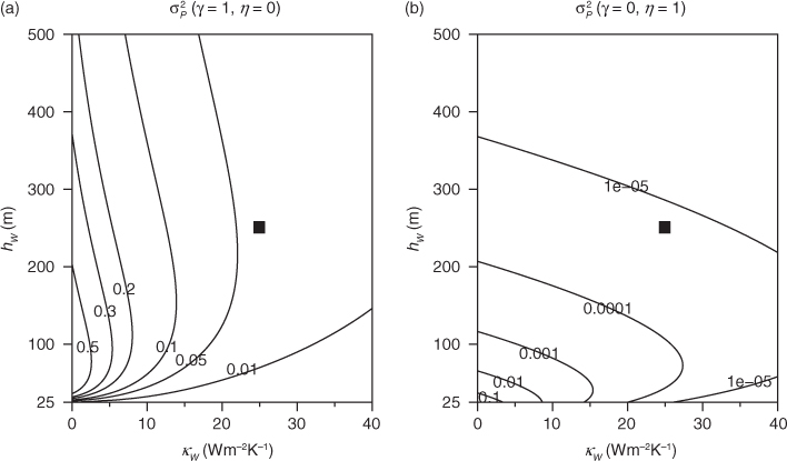
Fig. 8

4.2. The impact of varying κ_S and ${\sigma }_{Q_W}$ on ${\sigma }_{TW}^2$

As shown in Fig. 9a, ${\sigma }_{TW}^2$ varies little as the summer damping coefficient κ _S varies. The apparent greater sensitivity for larger h _W is due to the substantially reduced values of ${\sigma }_{TW}^2$ for larger h _W .

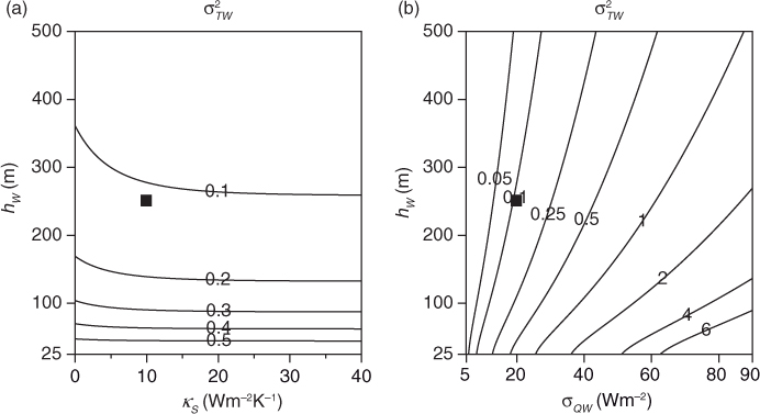
Fig. 9

Figure 9b quantifies the response of ${\sigma }_{T_W}^2$ to ${\sigma }_{Q_W}$. As expected, increasing the winter forcing ${\sigma }_{Q_W}$ increases ${\sigma }_{T_W}^2$ (roughly quadratically), by increasing present winter and previous winter temperature variances, with less sensitivity for larger h _W .

5.1. The effect of re-emergence and preceding winter temperature anomalies that persist in the summer mixed layer on P_W

The expression for the power spectrum of the winter temperature enables us to establish the influence of re-emergence, of preceding winter temperature anomalies that persist in the summer mixed layer, and of summer atmospheric forcing, for a range of timescales. Various winter spectra are illustrated in Fig. 10, using standard values.

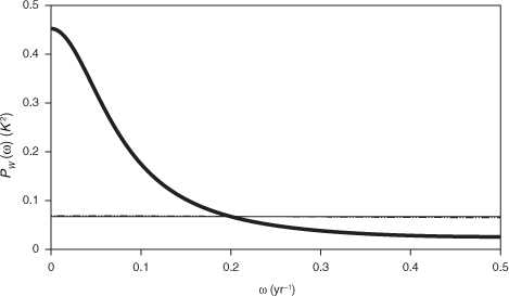
Fig. 10

When γ=η=0, $G_W(\omega )=1$ for all $\omega$, and eq. (29) reduces to $P_W(\omega ) = {\sigma }_R^2$. When there are no effects of re-emergence and preceding winter temperatures that persist in summer the power spectrum is flat, as shown by the thin black line in Fig. 10.

When η=0 and γ=1, C=f _W (1−r) in eq. (30) and only the effects of re-emergence influence P _W . This case is shown by the thick line in Fig. 10. The shape factor has G _W (0)=6.7, G _W (0.5)=0.4.

For γ=0 and η=1, C=rf _W f _S , and P _W is only influenced by preceding winter temperature anomalies that persist in the summer mixed layer. This case is illustrated by the broken line in Fig. 10: the effect of persistence on P _W is much weaker than that of re-emergence, as evident in the shape factor values G _W (0)=1.03, G _W (0.5)=0.97.

With persistence and re-emergence processes included (η=γ=1), for standard values the spectrum is very similar to that with re-emergence only. The graph for this case is included in the parameter comparisons shown in Fig. 11. Note that re-emergence reddens the winter temperature spectrum.

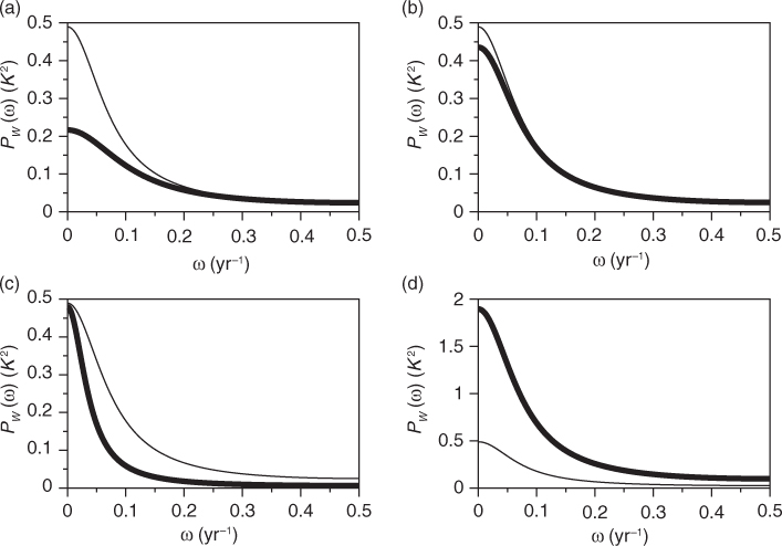
Fig. 11

Schneider and Cornuelle (2005) described spectra from numerical integrations with a similar two-season model, in which re-emergence increased the spectral power at interannual timescales but not at longer timescales. One reason for the contrast with our result is the experimental design. They compare spectra from an integration with a constant deep (winter) mixed layer with that from an integration with deep winter and shallow summer layers, whereas in our experiments there is always a deep winter and shallow summer layer and spectral comparisons are made by varying the ‘process flags’ and parameters. In their comparison, decreasing the summer mixed layer depth increases the variability of the mixed layer temperature in summer, which results in an increase in the spectral power of the mixed layer temperature at interannual and shorter timescales. A further difference is the throughout-season data sampling in Schneider and Cornuelle (2005) versus the end-of-season sampling in our results. An increase in spectral power at decadal timescales was also found in the study with idealised models by De Coëtlogon and Frankignoul (2003), in which they compared spectra from an integration with a constant e-folding scale of 3 months and an integration with the addition of a simple re-emergence term in winter.

5.2. The effect of varying κ_S, κ_W and h_W on P_W

In this section, the effect of varying κ _S , κ _W and h _W on P _W is investigated. Throughout this section, we set γ=η=1, and the reference case (represented by the thin lines in Fig. 11) uses standard values.

The thick line in Fig. 11a shows P _W when the winter atmospheric damping κ _W is increased to 40Wm⁻²K⁻¹. Increasing κ _W reduces ${\sigma }_R^2$, and also decreases C with the effect of flattening the shape of the spectrum. At interannual timescales these effects offset each other, and in this example the net result is very small [P _W (0.5) reduces from 0.025 to 0.024], whereas at decadal timescales the effects reinforce and the power is more than halved for P _W (0).

The thick line in Fig. 11b shows P _W when the summer atmospheric damping is increased to 40Wm⁻²K⁻¹. The system is less sensitive to κ _S , and in this case the power is reduced slightly.

The thick line in Fig. 11c shows P _W when the winter mixed layer depth is doubled to 500m. The term ${\sigma }_R^2$ is more than halved, but C is increased so the shape factor is steepened. The effects offset at long timescales, and the result in this case is a slight reduction of P _W (0) from 0.49 to 0.48. The effects re-inforce at interannual scales, and P _W (0.5) is reduced by about 75%.

Figure 11d shows how doubling ${\sigma }_{Q_W}$ (thick line) acts to increase the winter temperature variability at all timescales, by increasing ${\sigma }_R^2$ without affecting $G_W(\omega )$.

6.1. The impact of varying κ_W and h_W on Corr(T_W, T_S) and α

The effect of varying κ _W and h _W , with other parameters set to standard values and η=γ=1, is described here. The effect on the summer-to-following-winter correlation Corr(T _W , T _S ) is illustrated in Fig. 12a. As expected, for fixed h _W the correlation decreases as the winter damping κ _W increases. The correlation is small for h _W close to h _S except when winter damping is small: when winter depths are small the anomalies induced by the random winter forcing dominate the influence of previous seasons. The correlation then increases as h _W increases, then decreases: it is largest (over 0.4) for small κ _W and for h _W about 75 m. For the standard value κ _W =25Wm⁻²K⁻¹ correlation exceeds 0.2 for h _W ranging from 100 to 400 m. Comparing the pattern in Fig. 3b with that of Fig. 12a, it is clear that Corr(T _W , T _S ) is not as strongly influenced by variations in h _W as Corr(T _W , T _W−1).

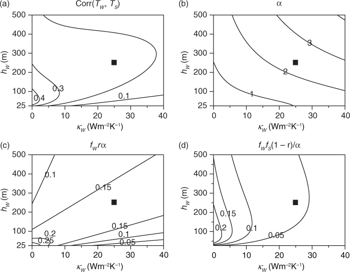
Fig. 12

As shown in Fig. 12b, the ratio ${\sigma }_{TS}/{\sigma }_{TW}$ increases as κ _W increases. As σ _TW decreases as winter damping increases, it is evident from eq. (31) that σ _TS also decreases but α increases as κ _W increases. Likewise the ratio also increases as h _W increases, because σ _TW decreases. For the parameter values used, the ratio is larger than 1 when h _W is larger than about 200 m when κ _W is small.

The contributions to the correlation from the two terms in eq. (35) are provided in Fig. 12c and d. In Fig. 12c the pattern is again linked to that of rf _W described in Section 3.1. For the ‘re-emergence’ term in Fig. 12d, this contribution is largest for small κ _W , with a maximum at around h _W =100 m for small κ _W . (The maximum is a result of the trade-off between increasing (1−r)f _W and decreasing $1/\alpha$ as h _W increases. As h _W increases, the amount of re-emerging water increases but the variance of its temperature decreases. This feature influences the occurrence and location of the maximum in correlation in Fig. 12a.) The two terms are similar in size: persistence of anomalies in surface layers and re-emergence of sub-surface information are both influential in the overall correlation between summer and following winter temperature anomalies. For the standard winter damping value κ _W =25Wm⁻²K⁻¹ re-emergence is less influential than the other term.

6.2. The impact of varying κ_S and h_W on Corr(T_W, T_S) and α

Similarly the effect of varying κ _S and h _W is illustrated in Fig. 13. In Fig. 13a it can be seen that Corr(T _W , T _S ) decreases as κ _S increases and summer anomalies are reduced. For h _W close to h _S the correlation is small (as in Fig. 12a). As h _W increases from h _S the correlation increases, and then weakly decreases for h _W larger than about 200 m. For low κ _S the correlation exceeds 0.4 for h _W between about 125 and 375 m. Comparing Fig. 3a with Fig. 13a, it is clear that Corr(T _W , T _S ) is more sensitive to variations in κ _S than Corr(T _W , T _W−1).

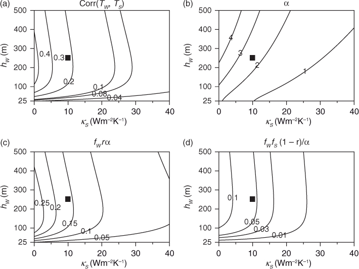
Fig. 13

The ratio α, shown in Fig. 13b, decreases as κ _S increases: while increasing the summer damping reduces both summer and winter variances, the more direct effect on the summer variance is greater. Similar to Fig. 12b, for fixed κ _S the ratio increases as h _W increases and winter variances decrease. Small κ _S favours larger summer variance, and α is largest for low κ _S and large h _W .

The components of the correlation are provided in Fig. 13c and d. For small fixed κ _S the term f _W rα in Fig. 13c has a maximum at h _W about 200 m. This contrast to the pattern in Fig. 12c occurs because α now increases as h _W increases. Both terms have similar behaviour as κ _S and h _W vary, with f _W rα generally more than twice the re-emergence contribution.

6.3. The impact of varying σ_QW on Corr(T_W, T_S) and α

Changing the winter forcing standard deviation σ _QW changes the winter temperature variance correspondingly. The effect on Corr(T _W , T _S ) and α is explored here by varying σ _QW and h _W with other parameters set to their default values. (Note that the default for σ _QS is 10Wm⁻², the default for σ _QW is 20 Wm⁻², and σ _QW ranges from 5 to 90 Wm⁻² in the results illustrated.)

Figure 14a shows Corr(T _W , T _S ). For small σ _QW the random forcing of winter anomalies is weak and anomalies from the previous summer can have a stronger influence: thus the largest values in Fig. 14a occur with σ _QW at the low end of the range, reaching about 0.5 when h _W is in the range 100–250 m. As σ _QW increases from 5 Wm⁻² the correlations decrease at first, but then increase again for σ _QW larger than 40 Wm⁻². The reason is that the re-emergence contribution to the correlation increases as σ _QW increases and winter variance increases. This is clear from the two contributions to the correlation mapped in Fig. 14c and d: for small σ _QW f _W rα in Fig. 14c dominates, while for large σ _QW $f_W{f}_S(1-r)/\alpha$ dominates.

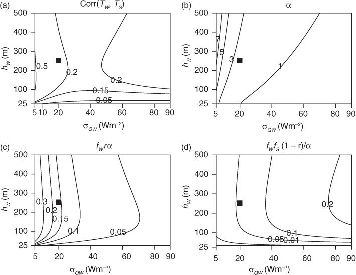
Fig. 14

This behaviour is related to the effect of σ _QW on α shown in Fig. 14b. Decreasing σ _QW decreases both σ _TW and σ _TS , but the effect is relatively larger for σ _TW . Consequently the ratio α increases markedly as σ _QW decreases below about 20 Wm⁻², particularly for larger h _W . Increasing σ _QW above the default value of 20 Wm⁻² has a weak decreasing effect on α.

For h _W close to h _S the correlation is weak for all σ _QW in the example.

7.1. The response of R and R^* to varying κ_W, κ_S and σ_QW

Unless otherwise stated, parameters have their default values and η=γ=1. Figure 15a and b show R and R ^* when κ _W and h _W are varied and other parameters have their default values. R and R ^* have similar relatively low values for h _W close to h _S , and increase as h _W increases. R is not very sensitive to κ _W , whereas R ^* increases more rapidly with depth when κ _W is small. For small winter damping κ _W winter temperature variance is relatively large and re-emergence has a stronger effect, and this influence is emphasised in R ^*.

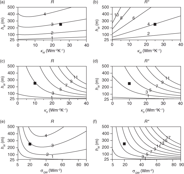
Fig. 15

As seen in Fig. 15c and d the effect of varying summer damping κ _S is very similar for R and R ^*. In this example the largest values are found for large h _W and large κ _S , because summer temperature anomalies are strongly damped by large κ _S and re-emergence again has a stronger effect.

The effect of varying winter forcing σ _QW is illustrated in Fig. 15e and f. Differences between R and R ^* are most evident for larger σ _QW . For σ _QW larger than 40Wm⁻², R decreases but R ^* increases markedly as σ _QW increases. This occurs because winter temperature variance increases as σ _QW increases: the re-emergence component maintains Corr(T _W , T _S ) in R (cf. Fig. 14a), while Corr(T _W , Q _S ) decreases in R ^*.

8.1. The summer-to-summer correlation

As derived in the Appendix, the summer-to-summer correlation is

When η=0, Corr(T _S , T _S−1)=0, that is, preceding summer temperatures cannot influence the summer temperature if winter temperatures do not influence the summer temperature. (a), (b) and (c) of Fig. 16 show how Corr(T _S , T _S−1) varies with h _W , κ _W , κ _S and σ _QW with other parameters in each figure set to their default values. It is clear that, as expected, preceding summer temperatures have little influence on those in the following summer for the ranges of parameters considered here.

Fig. 16

8.2. The power spectrum of the summer temperature

As derived in the Appendix, the power spectrum of the summer temperature is

where

and

When η=0 successive summers are uncorrelated and $P_S(\omega )={\sigma }_{T_S}^2$.

Figure 17 shows $P_S(\omega )$ for standard values (thin line) and for some parameter variations (cf. the winter spectra in Fig. 11). For standard values the spectrum is weakly red. Increasing the winter damping rate κ _W to 40Wm⁻²K⁻¹ reduces the winter temperature anomalies that persist into summer, flattening the spectrum (Fig. 17a). Increasing the summer damping rate κ _S to 40Wm⁻²K⁻¹ reduces the summer variance considerably (Fig. 17b). Doubling the winter depth h _W increases the power at interannual scales and reduces it at decadal scales (Fig. 17c). Doubling the winter forcing σ _QW increases the power slightly, more so at low frequencies (Fig. 17d).

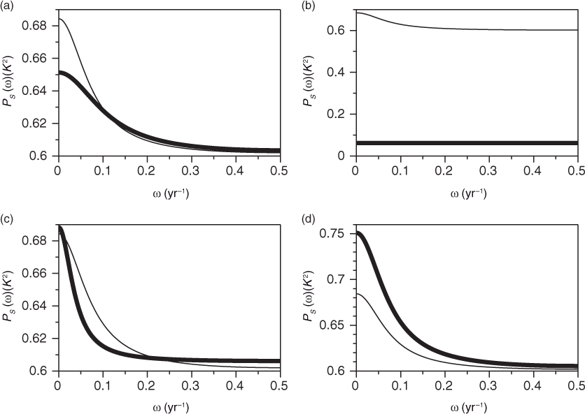
Fig. 17