

Fig. 1
RMSE of the analysis ensemble mean [eq. (8)] when using the composite state method (CSM). Bias correction (blue curve) significantly increases the analysis accuracy compared with the analysis without bias correction (red curve), and approaches perfect (unbiased) global forecast model results (black curve). The inset figure plots the spatial dependence of the time-averaged estimated bias correction b (gold curve) and the estimate provided by eq. (9) (green curve).
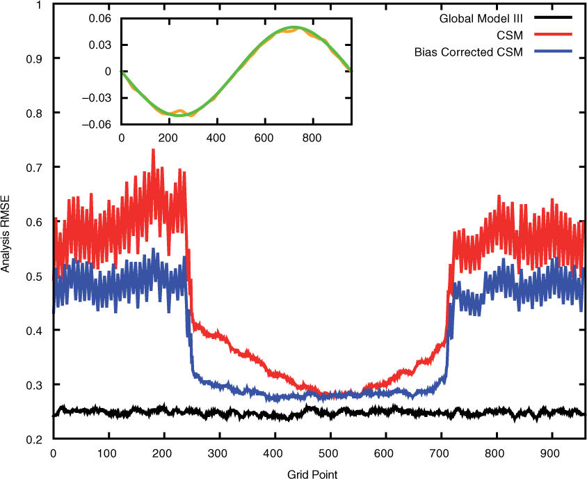
Fig. 2
Same as Fig. 1, but with spatially dependent bias ΔF. Bias correction leads to decreased analysis RMSE compared to the composite state analysis without bias correction (blue versus red curves, respectively). The inset figure shows averaged bias correction b (gold curve) versus the value predicted by eq. (9) (green curve).
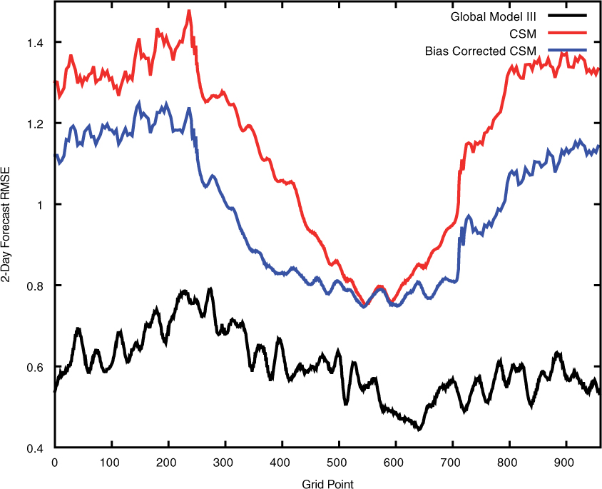
Fig. 3
RMSE of 2-d forecast ensemble mean, for spatially dependent bias as in Fig. 2. Blue and red curves compare forecasts with and without bias correction, respectively. The black curve shows ensemble forecast RMSE when forecasting with the truth model.