
Table 1. List of schemes used in 1D case study
First-order FDNoneSecond-order Lax-WendroffNoneThird-order FDNonePPMNonePPMColella and Woodward (1984)CWPPMColella and Sekora (2008)CSPPMColella and Woodward (1984) + Lin (2004)CWLThird-order FDLeonard (1991) (universal)ULSLICENoneSLICEBermejo and Staniforth (1992)BES
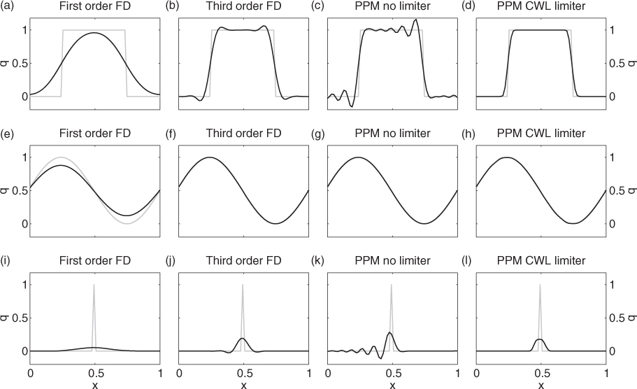
Fig. 1
Advection, once around the domain, of the step function (top row), the sine function (middle row) and the point function (bottom row). The first-order finite difference scheme is shown in panels (a, e and i). The third-order finite difference scheme is shown in panels (b, f and j). The unlimited PPM scheme is shown in (c, g and k). The PPM with CWL limiter is shown in (d, h and l). The grey curve shows the exact solution (equal to the initial conditions for this simple case). The black curves show the result when using the different schemes.
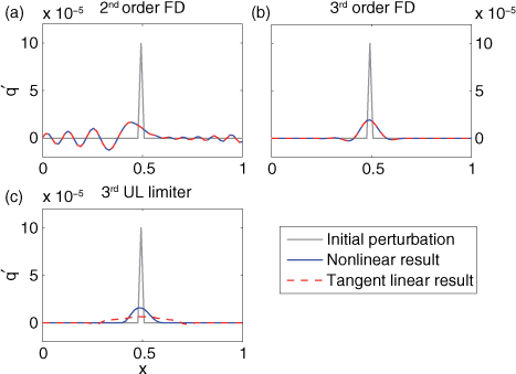
Fig. 2
Comparison of the initial perturbation (also the truth solution), the non-linear perturbation trajectory (blue) and the linear perturbation trajectory (red dash) when perturbing the step function initial conditions with a point perturbation.
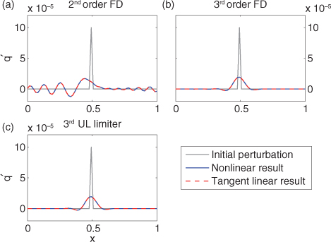
Fig. 3
As for Fig. 2 but when perturbing the sine wave initial condition with the point perturbation.
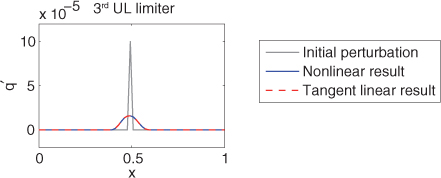
Fig. 4
As for Fig. 2c but when perturbing the point function initial conditions with the point perturbation.
Table 2. The root mean square error between the tangent linear perturbation and the exact perturbation (linear schemes are zero), the correlations between the tangent linear perturbation and the non-linear perturbation (linear schemes are one) and the normalised root mean square error of non-linear perturbation and the tangent linear perturbation (linear schemes are zero)
Third-order UL1.20×10−51.10×10−51.12×10−5PPM CW3.38×10−51.10×10−51.11×10−5PPM CS1.44×10−51.10×10−51.14×10−5PPM CWL3.20×10−31.10×10−51.12×10−5SLICE BES1.25×10−31.10×10−51.12×10−5CorrelationsStep functionSine functionPoint functionThird-order UL0.761.001.00PPM CW0.190.991.00PPM CS0.530.931.00PPM CWL1.41×10−31.001.00SLICE BES3.64×10−81.001.00 Grad testStep functionSine functionPoint functionThird-order UL1.0––PPM CW1.01.10×10−2–PPM CS0.850.40–PPM CWL1.05.5×10−5–SLICE BES12.3––
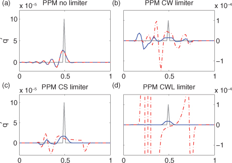
Fig. 5
As for Fig. 2 but for the PPM type schemes.
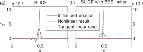
Fig. 6
As for Fig. 2 but for the SLICE schemes.
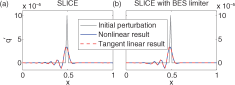
Fig. 7
As for Fig. 6 but perturbing the sine wave initial conditions.
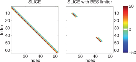
Fig. 8
Jacobian of the SLICE scheme and SLICE with BES limiter scheme at time step 292.
Table 3. List of non-linear schemes with the average, over all time steps, of the eigenvalue with largest real part and the percentage of time steps for which an eigenvalue with a positive real part occurs
Third-order UL limiter8.1061.09PPM with CW limiter7.71100PPM with CS limiter48.71100PPM with CWL limiter60.70100SLICE BES limiter0.000.00
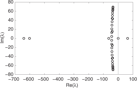
Fig. 9
Complex plane scatter plot showing the eigenvalues for the third-order scheme with UL limiter. The eigenvalues are computed for time step 292.
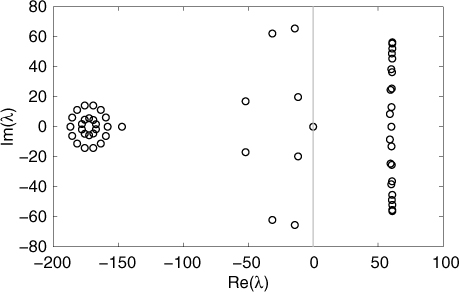
Fig. 10
As for Fig. 9 but for the PPM scheme with CWL limiter.
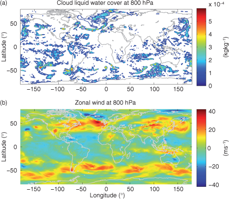
Fig. 11
Upper panel shows the cloud liquid water field at the 800 hPa height. The lower panel shows the zonal component of wind at 800 hPa.
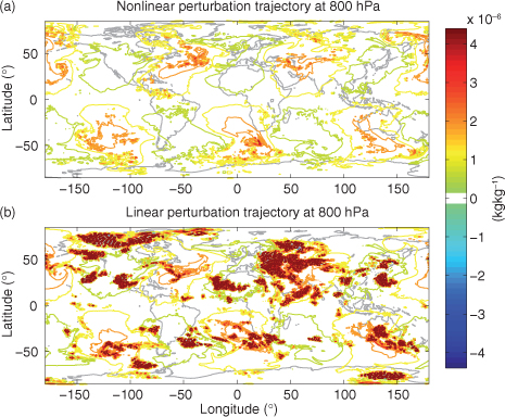
Fig. 12
Upper panel shows the non-linear perturbation trajectory when using the CWL limiter at the 800 hPa height. The lower panel shows the equivalent tangent linear perturbation. The contour interval is 6×10⁻⁷.
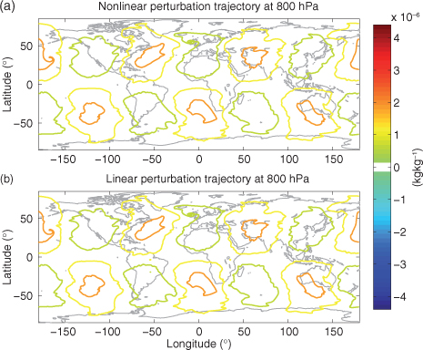
Fig. 13
As for Fig. 12 but showing the result when using the third-order finite difference scheme in both the non-linear and tangent linear models.
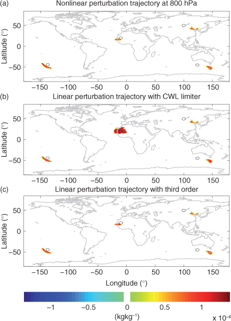
Fig. 14
The top panel shows the non-linear perturbation trajectory at the 800 hPa height when perturbing the cloud liquid water using the cylinder functions. The middle panel shows the linear perturbation trajectory when using the CWL limiter. The lowest panel shows the linear perturbation when using the third-order scheme in the tangent linear model. The black curves show the outline of the initial cylinder functions. The contour interval is 2×10⁻⁷.
Table 4. Root mean square errors for the cylinder perturbations when using the PPM scheme with CWL limiter and the third-order finite difference scheme
(−138°, −44.5°)1.783×10−71.566×10−7(−10°, 20°)1.169×10−62.489×10−8(100°, 50°)1.242×10−71.269×10−7(124°, −45°)8.420×10−86.910×10−7
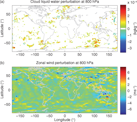
Fig. 15
The initial cloud liquid water perturbation (top) and zonal wind perturbation (bottom), plotted with a contour interval of 5×10⁻⁵ and 0.7.
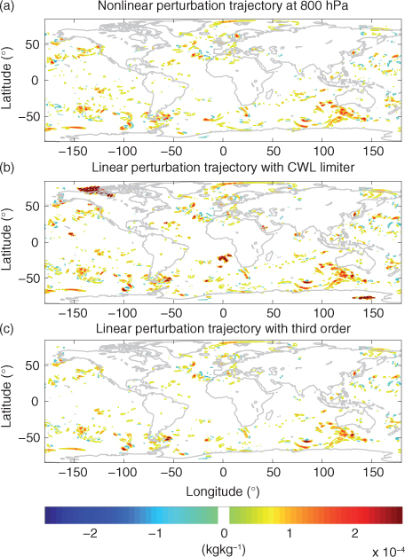
Fig. 16
As for Fig. 14 but showing the cloud liquid water perturbation trajectories when using the analysis increment initial condition. The contour interval is 5×10⁻⁵.
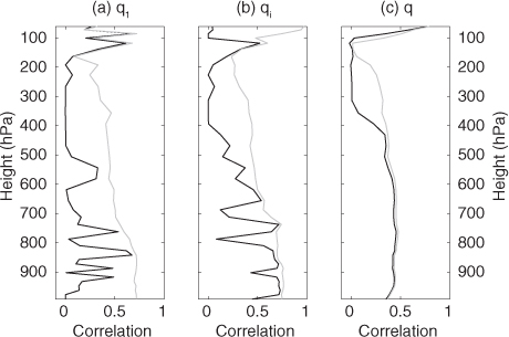
Fig. 17
Global correlations between the linear and non-linear perturbation trajectories plotted as a function of pressure. The black curve shows the correlation for the CWL-limited scheme, and the grey curve shows the correlation when using the third-order scheme. The left panel shows the correlations for cloud liquid water, the middle panel for cloud liquid ice and the right panel for specific humidity.