
Table 1. Some cyclonic windstorms that have affected Europe
ISD storms
Daria25/01/90UK,NL,DKW C1990); McCallum (1990)Vivian26/02/90IE,UK,DE,BE,CH,AT,NLW C1990)‘Venice92’09/12/92ITW–Lili (ET)28/10/96IE,UK,DEC2005)Yuma24/12/97IE,UK(S) C1999)Anatol03/12/99DE,DK,SES C2001); Nielsen and Sass (2003)Lothar26/12/99FR,CH,DE,ATW (S)2001); Wernli et al. (2002)Martin28/12/99FR,CH,DEC2001)Oratia30/10/00UKW S C2001)Torsten11/11/01DZ,ESC2005)Jeanette27/10/02UK,NL,BE,DE,PL,CZC2009)Quimburga20/11/04CZ,AT,SK(W) C2009)Dagmar17/12/04FRC2007)Erwin08/01/05UK,DK,SE,EEW S C2009)Gordon (ET)20/09/06ES,IE,UK(W) C2008)Renate03/10/06FRS CIbidKyrill18/10/07UK,DE,CH,AT,DE,PL,CZW C2009)Paulaa25/01/08DE,PL,CZ,ATW C Joyner (2013) Klaus24/01/09PT,ES,FRC Liberato et al. (2011); Bertotti et al. (2012) Xola23/12/09PTS C Pinto and Silva (2010) Xynthia28/02/10FR,DE(S) C Lumbroso and Vinet (2011) Ulli03/01/12UKS C Fox et al. (2012); Smart and Browning (2014) Other storms
‘October87’15/10/87UK,FRS C1988); Shutts (1990); Browning (2004)Herta03/02/90FR,BE,DE(S) C1990)Petra15/07/10UKS Wales Online (2010) Friedhelm08/12/11UKC Baker et al. (2013); Vaughan et al. (2014) Christian28/10/13UK,NE,DK,DE,SES C Hewson et al. (2014) Xaver05/12/13UK,NE,DK,DEC Hewson et al. (2014) Ulla14/02/14UK,FRW C
[i] List of cyclonic windstorms, in the IMILAST dataset (ISD, top section) and others discussed in this paper (lower section). ET denotes extra-tropical transition case. The likely cause(s) of the strongest gusts over land, according to the framework of Fig. 1, are given in the fourth column: W for the warm jet, C for the cold jet and S for the sting jet. Methods of assignation are discussed in the text. Confidence therein is limited by available data, and is subjectively assessed – parentheses indicate ‘probable’ (50–90% confidence), whilst no parentheses signify ‘very probable’ (>90% confidence). aNote that damage historically attributed to Paula relates in fact to two cyclones, the one named by the Free University of Berlin that ran east into Scandinavia, and a wave depression that developed later, on its southern flank, over southern Scandinavia, that was not named.
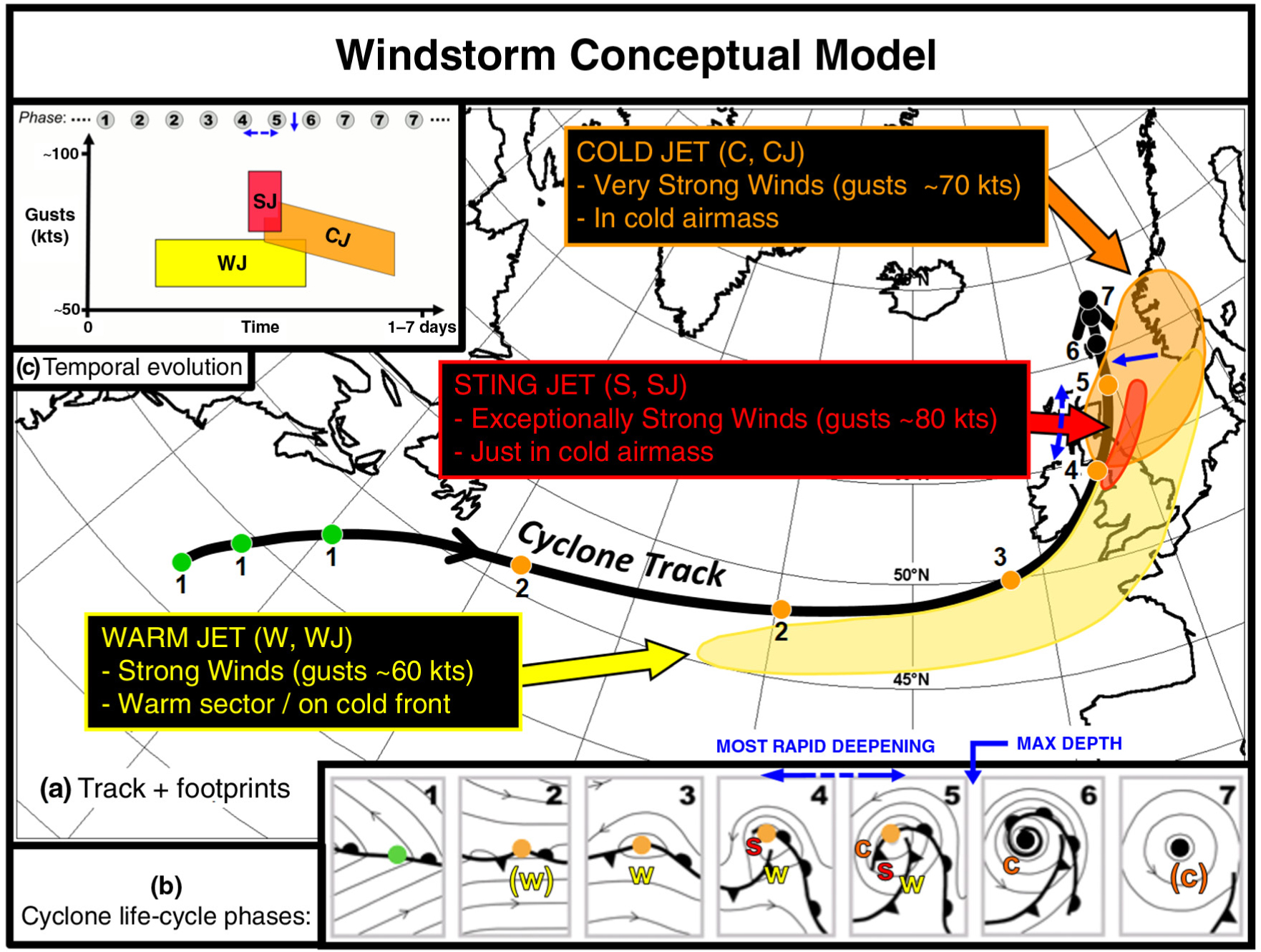
Fig. 1
Conceptual model of an extra-tropical cyclonic windstorm. Panel (a) shows the cyclone track (black), with spots denoting positions equally separated in time, and numbered according to the cyclone life-cycle phases in panel (b). Spot colour relates to the identification method and objective typing used in Hewson and Titley (2010), green being a diminutive frontal wave, orange a frontal wave cyclone, and black a barotropic low. Shading denotes the footprints, or nominal damage swathes, attributable to the warm jet/warm conveyor (yellow), the cold jet/cold conveyor (orange) and the sting jet (red). Panel (b) shows the synoptic-scale evolution of fronts and isobars around the cyclone, after Hewson and Titley (2010) and Shapiro and Keyser (1990), with added letters denoting relative locations of the strong wind features, and brackets indicating marginal existence. Panel (c) denotes the temporal evolution of gust strength for each jet zone, with numbers cross-referencing phases on panel (b). On each panel, a dashed blue line denotes the period of most rapid deepening, whilst the solid blue arrow shows the time of maximum depth. This conceptual model should be considered to be very malleable; for example most intense cyclones will have only one or two of the three strong wind footprints associated.
Table 2. Key characteristics of windstorms, based around the conceptual model shown in Fig. 1
Location of strong winds (relative to cyclone and fronts)Between warm and cold fronts, and on the cold front itself.Near to the tip of the bent back front, extending NE, E or SE towards the region of frontal fracture.In cold air encircling the low, initially on the W flank, but moving on with time to the SW, S and SE flanks.Approximate timing of strong windsRelatively early in the life cycle, but on the cold front somewhat later. Disappears as warm air occludes.During and just after the period of most rapid cyclone intensification.Starts out just prior to the time of maximum cyclone depth, then decays slowly.Duration of very strong winds~24–48 hours~1–12 hours~12–36 hoursRelative frequencyFairly unusualVery rareFairly commonStability characteristicsMostly stable, but pockets of low to mid-level instability possible in warm sector or along cold front.Cooling through evaporation of cloud head particulate is believed to enhance an instability to downward slantwise convection.Unstable along onshore coasts; more stable inland, though prone to destabilise here through insolation.Inland versus coastal sitesStronger gusts on windward coasts where friction lower. Stability effects reduce strength at all sites, though embedded convection can complicate.Unrelated, due to top-down destabilisation mechanism. So very probably the main driver of extreme gusts inland.Much stronger gusts on coasts, due to marine (SST-derived) instability. However, insolation may create similar conditions inland by day.Typical relative wind strengths (but can vary)VGUST<<V1KM, V1KM~VGVGUST~V1KM, V1KM~VGVGUST<V1KM, V1KM<VGAccompanying weatherMostly cloudy, rain and drizzle possible, heavier in any embedded convection and on cold front.Largely dry, broken cloud expected.Showers likely near windward coasts, possible inland. Cloud usually broken. But thick cloud and heavy rain possible in early stages (cloud head).Footprint width~200–500 km (less significant inland)~20–200 km~100–800 km (may be less significant inland)Footprint length (over land)Up to ~1000 kmUp to ~800 kmUp to ~2500 kmEase of predictionUsually straightforward (though cold front gusts more problematic).Very difficult.Relatively straightforward, though stability impact can be difficult to gauge.Gusts represented in ERA-Interim?Yes, generallyNoOK but some weaknesses, especially early on and for smaller systems.
[i] Summary of key characteristics of the three windstorm phenomena shown on Fig. 1, as deduced primarily from the cases in Table 1. VGUST is wind gust strength, V1KM is the wind speed 1 km above the earth's surface and VG is the near-surface geostrophic wind speed. Note that the ‘Relative frequency’ row in the table is intended to be a rough guideline spanning all European cyclones; this differs from the impression given by Table 1 because that shows only pre-selected extreme cases. Characteristics are further discussed in the text.
Table 3. How the causes of peak gusts over land were assigned
1.Refer to BESTTRK data to ascertain cyclone timing.2.Examine surface observations (from various sources*) over land to ascertain peak gusts associated with the cyclone (referencing step 1) and the times when they occurred.3.Obtain (from various sources**) synoptic chart sequences at ≤6 h intervals, to span the time of the peak gusts (from step 2), in order to document where, relative to front and cyclone positions, the peak gusts occurred.4.Assign each of the peak gusts to one of the following three categories:
WJ: If the gust was in the warm sector or on the cold front (stages 2,3,4,5 on Fig. 1b).
CJ: If the gust was in the cold air behind the cold front and either (1) this gust was situated more than 300 km from the tip of a bent back front/occlusion or frontal wave, and/or (2) the bent back front/occlusion extended more than 300° around the low centre, as measured from the bearing of the triple point. (5, 6, 7 on Fig. 1b)
CJorSJ: If the gust was in the cold air behind the cold front, and neither (1) nor (2) immediately above were satisfied.5.For cases in the ‘CJ or SJ’ category investigate in detail whether a SJ was the likely cause, using wide-ranging data, as available, and following the detailed guidelines regarding SJ hallmarks presented in Section 3.3. Accordingly where SJ probability is subjectively deemed to be greater than 50% assign SJ as the cause, otherwise assign CJ.
[i] Shows the process by which the causes of peak gusts over land (WJ, SJ, CJ) for the windstorm-generating cyclones examined for this paper (Table 1) were ascertained. At step 2 the data sources (*) included standard observations circulated in real time via the global telecommunications system (GTS), observations documented in references on Table 1, autographic records obtained separately (e.g. Fig. 9b), and observational evidence documented on web sites (e.g. www.meteo-paris.com/chronique/annee/yyyy, where yyyy is the year). At step 3 sources (**) included Met Office surface analyses (recent years online at www2.wetter3.de/Archiv/archiv_ukmet.html), surface analyses from references in Table 1, analyses drawn manually for this paper, and objective synoptic charts from the ECMWF model (based on Hewson, 1998).
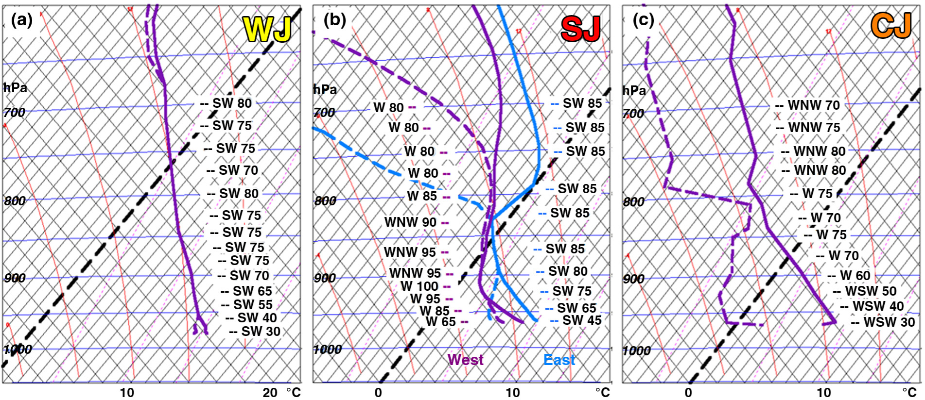
Fig. 2
Example UK-area lower tropospheric soundings for the WJ, SJ and CJ phenomena, in (a), (b) and (c), respectively, with winds in alphanumeric format (speeds in kts). Pressure in hPa is shown on the left, whilst temperature in °C is shown below. (a) is for Camborne at 00 UTC on 30 October 2000 (Oratia), whilst (c) is for Crawley at 18 UTC on 25 January 1990 (Daria). To denote the SJ (b) shows two soundings from ECMWF HRES 6-hour forecast fields valid at 06 UTC on 3 January 2012 (Ulli). These nominally straddle the SJ surface impact zone at this time; mauve is to the west, blue to the east. Sounding locations are shown (by coloured rings) on Fig. 4b for the WJ in (a), on Fig. 10b for the SJ in (b), and on Fig. 4a for the CJ in (c).
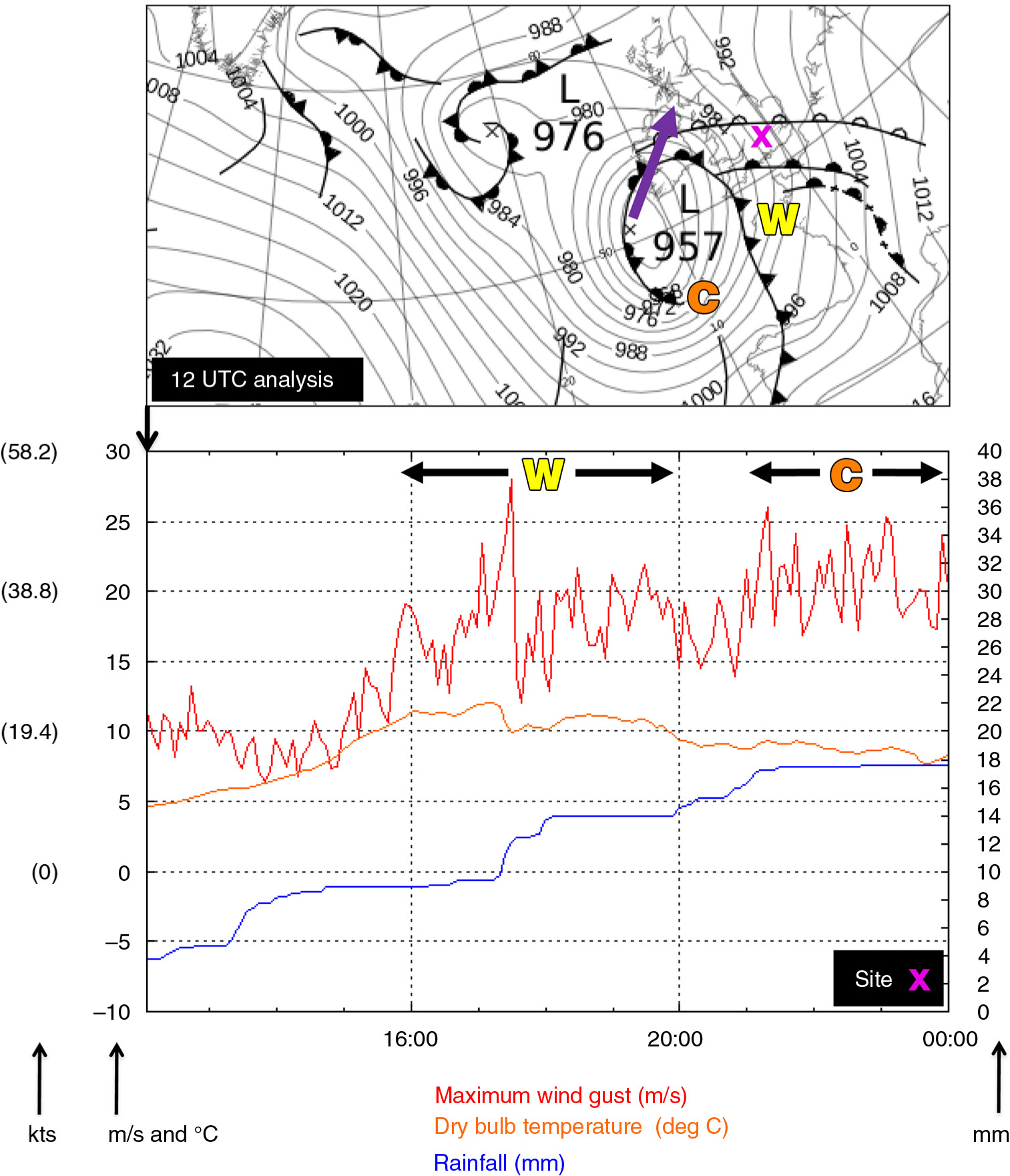
Fig. 3
Top panel shows a portion of the Met Office synoptic analysis chart for 12 UTC on 14 February 2014; Ulla (Table 1) is the cyclone southwest of Ireland. A purple arrow shows the 12-hour movement of Ulla whilst ‘W’ and ‘C’ denote the centres of, respectively, the WJ and CJ phenomena at 12 UTC. A pink cross marks the Reading University Atmospheric Observatory. Panel below shows observations from this Reading site for the same date, as Ulla advanced northeastwards. Red shows gust strength (m/s and kts, left axis), blue shows accumulating rainfall total for the day (mm, right axis) and orange shows screen temperature (°C, left axis). Time on the x-axis is UTC. Labelling at the top denotes the approximate durations of the warm and cold jet phenomena at this site, as inferred from the traces and synoptic pattern. (The lower panel is reproduced with permission from Reading University Department of Meteorology).

Fig. 4
Maximum wind gusts (kts) observed during the passage of three ISD cyclones (Table 1); Daria in (a), Oratia in (b) and Renate in (c). Letters denote the assigned cause of the maximum gust in different regions (W for warm jet, S for sting jet and C for cold jet). Orange and yellow rings on (a) and (b) respectively denote the locations of Camborne and Crawley; soundings from these sites for the said windstorms are shown on Fig. 2c and 2a, respectively. (Panels a and b are reproduced with permission from the Met Office).
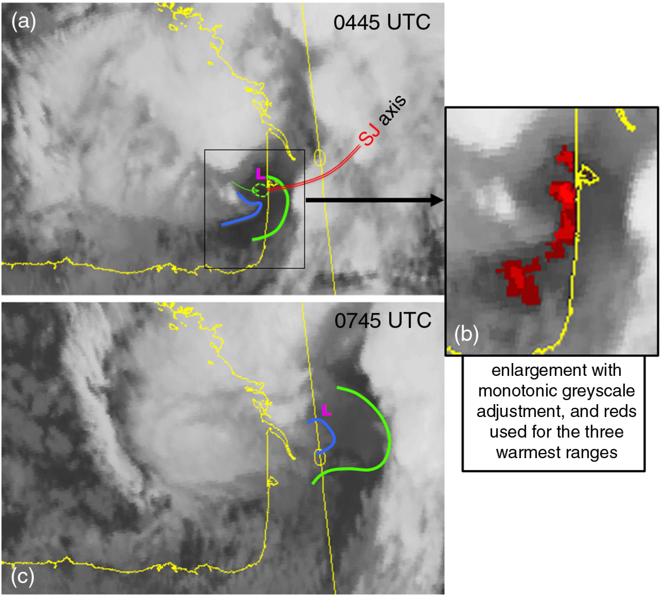
Fig. 5
Meteosat infra-red images during the passage of windstorm Renate (Table 1) on 3 October 2006, at 0445 UTC (a), with an enlarged portion in (b), and 0745 UTC (c). L denotes the low centre and the blue line denotes the evolving edge of the cloud head tip. The solid green line denotes the forward edge of an advancing low-level cloud sheet which had breaks in at the earlier time; the closed dashed green contour highlights the most clear-cut break [brightest red on (b)]. The green arrow aligns with a gap/furrow of warmer cloud tops in the cloud head. This furrow is believed to be symptomatic of a descending pulse of high momentum air – the SJ – that is moving in the direction of the arrow, faster than the low centre is moving. The double red line is the axis along which the maximum SJ gusts occurred (from Fig. 4c).
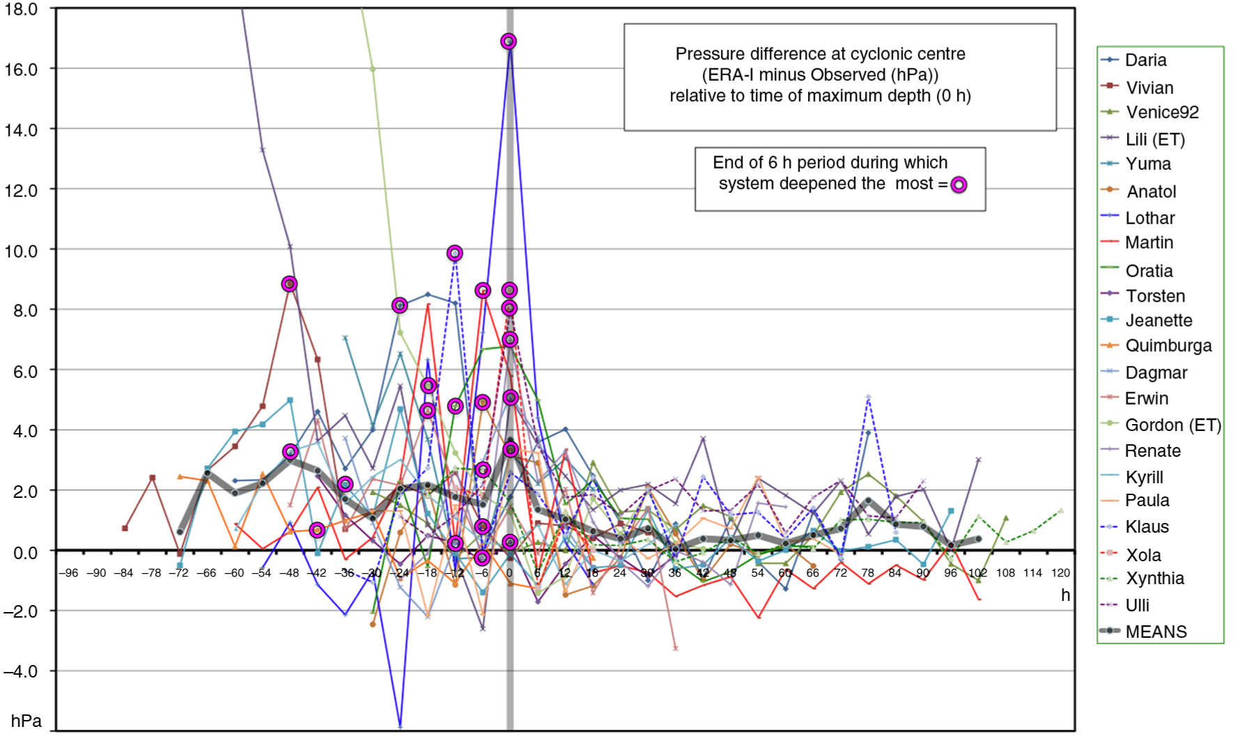
Fig. 6
Differences between cyclone central pressure in ERA-Interim (ERATRK) and in the best-track dataset (BESTTRK), in hPa, for each IMILAST windstorm (see legend). The x-axis shows hours relative to the (best-track) time of maximum depth for each cyclone. The thick grey line denotes mean behaviour (plotted only when at least three cyclones contributed). Pink rings denote the end of the 6-hour period during which the cyclone deepened the most (BESTTRK). For the two extra-tropical transition cases (ET in legend) only the extra-tropical phase was considered when identifying the times of maximum depth and maximum deepening.
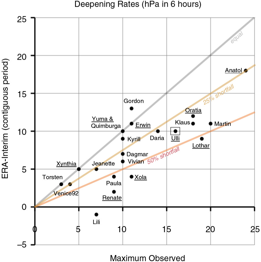
Fig. 7
Maximum observed 6-hour deepening (=change in central pressure) for the ISD cyclones, in hPa, compared to the 6-hour cyclone deepening shown by ERA-Interim over a contiguous period. Diagonal lines are shown as a guide, signifying the degree of shortfall in ERA-Interim. Underlining of storm names denotes that the storm was believed to have a sting jet footprint associated over land (as on Table 1). A box highlights the Ulli cyclone discussed in Section 4.
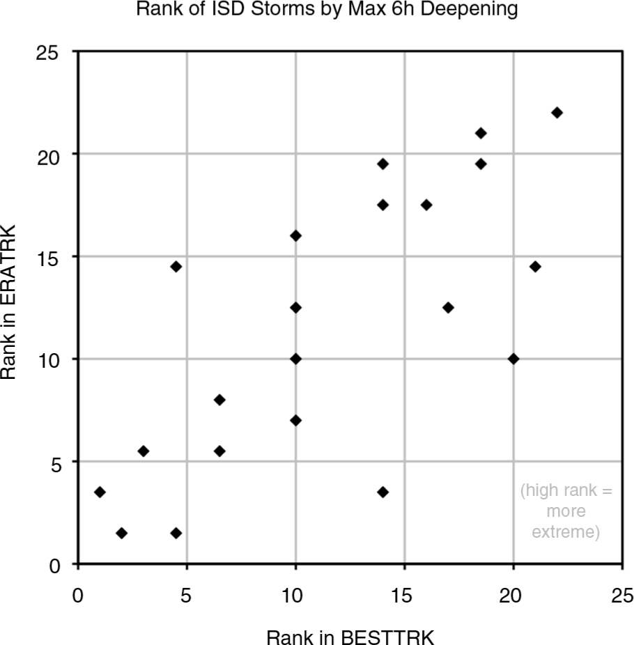
Fig. 8
Relative ranks of the 22 ISD storms in BESTTRK (x-axis) and ERATRK (y-axis) using maximum 6-hour deepening during each cyclone's life-cycle as the metric. Higher ranks denote more extreme deepening. The tropical phases for the two ET cases were discounted.

Fig. 9
Observational data for cyclone Ulli that hit Scotland on 3 January 2012 (Table 1). Panel (a) shows maximum reported gusts that day in kts. Orange and red outlines denote the areas of influence of the CJ and SJ, respectively (as on Fig. 1a). These were deduced from surface observations and from signatures on a 5-minute interval satellite image sequence, both of which were cross-referenced with mean sea level pressure, maximum gust, precipitation rate and simulated cloud fields from an operational run of the Met Office's UK4 model with a nominal data time of 21 UTC on 2nd (this run is also represented on Fig. 10c and d). An arrow points to the Glasgow Bishopton site. Panel (b) shows 1 minute maximum gust observations from this site, in kts, between 3 and 12 UTC on 3rd. Panel (c) shows an infra-red image for the time of the maximum gust at Bishopton. Green arrows denote two gaps between cloud head tips/fingers that retained their identities on the image sequence. The northern one is believed to relate to the sting jet maximum gust arrowed on panel (b), the site is shown (nearby) with a red dot. Note that parallax errors exist due to the remoteness of the subsatellite point (0°N, 7.5°E). The inset is a duplicate with coasts added. (Observations on panels a and b are reproduced with permission from the Met Office).
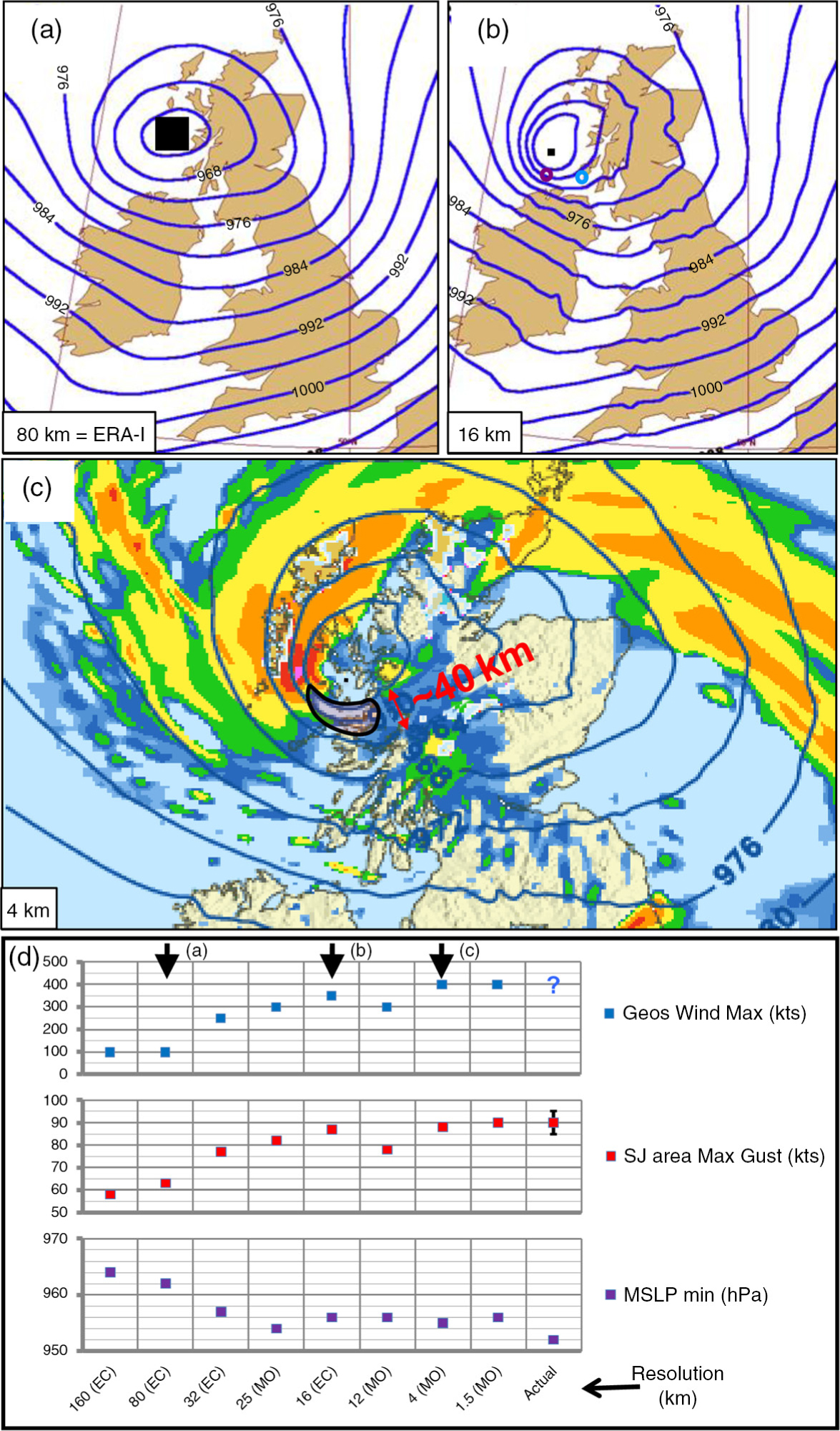
Fig. 10
Numerical model representations of IMILAST cyclone Ulli (Table 1) on 3 January 2012. Panels (a) and (b) show, for 06 UTC on 3rd, mean sea level pressure in hPa from, respectively, the ERA-Interim re-analysis (80 km resolution) and the 6-hour ECMWF HRES (high-resolution, 16 km) forecast. Panel (c) shows, for 08 UTC on 3rd, from the Met Office UK4 model run with a nominal data time of 21 UTC on 2nd, mean sea level pressure contours in hPa, precipitation rate in colour (blue, green, yellow, orange, red, pink denote 0.1–1, 1–2, 2–4, 4–8, 8–16, 16–32 mm/hr, respectively; lighter shades with a pale blue outline denote snow) and an 80 kt gust isotach (black). On each of panels (a, b, c) a black box near the cyclone centre shows effective model gridbox size. Coloured rings on (b) denote the locations of model soundings shown in Fig. 2b. Panel (d) compares three windstorm metrics – the cyclone central pressure (hPa, purple), the maximum sting jet gusts (kts, red) and the maximum geostrophic wind (kts, blue), at 06 UTC on 3rd, as represented in various Met Office (MO) and ECMWF (EC) operational forecast runs and re-analyses (labelled below with horizontal resolution given in km). Actual denotes observations. Data sparseness makes measuring the actual maximum geostrophic wind impossible though metric match up with the higher resolution models suggests that it was about 400 kts. The leftmost model is ERA-Interim data extracted at lower resolution (160 km); climatological results in Neu et al. (2013) used input data at this resolution. Arrows highlight the models shown in panels (a,b,c). (Panel c is reproduced with permission from the Met Office).
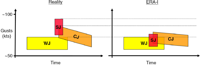
Fig. 11
Schematic showing how ERA-Interim's representation of 10 m wind gusts over land during the passage of a cyclonic windstorm (right side) typically compares with observed values (left side). WJ, SJ and CJ are, respectively, the warm jet, sting jet and cold jet phenomena (see Fig. 1).
Table 4. IMILAST experiments in the period 2009–2015, in chronological order
1Re-analysis, ERA-I, 1.5° resolution1989–2009NH, SH15Neu et al. (2013)2Climate model, ECHAM5/OM1, A1B scenario1961–2000; 2061–2100NH11Ulbrich et al. (2013)3Re-analysis, ERA-I, 0.75° resolutionSingle stormsNorth Atlantic & Europe12TELLUS special issue4Re-analysis, ERA-I, 1.5° resolution1979–2009NH, SH14TELLUS special issue