
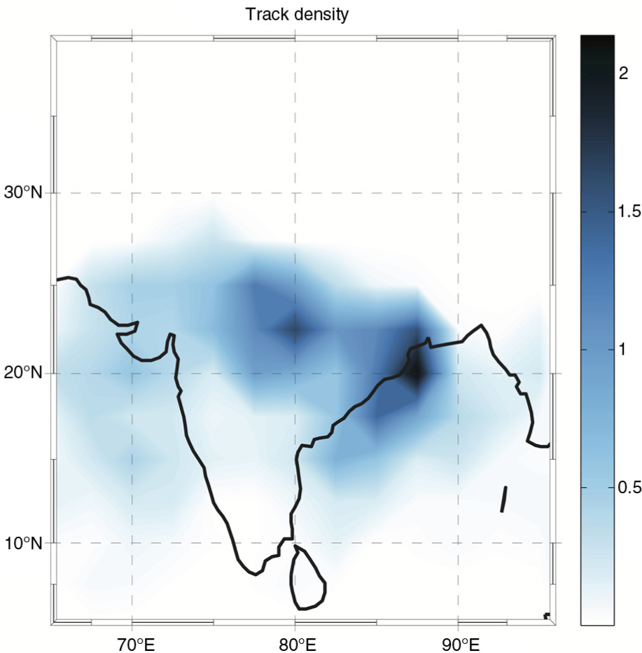
Fig. 1
The track density is showing the trajectories obtained from the algorithm, where the average number of trajectories during the monsoon season (LPS) is counted within a 2.5° square box. The time period used is 1979–2010.
Table 1. All the different criteria used to detect the monsoon LPS in the ERA-interim re-analysis data set by using the automated tracking algorithm
Vorticity intensityThe T42 relative vorticity at 850 hPa>0.5×10⁻⁵ s−1Lifetime and displacementMinimum 5° displacement during the lifetime. The minimum lifetime is 48 h (8 time steps)A true MSLP minimumA MSLP minimum (within a radius of 5° around the feature points) must exist for at least four consecutive time stepsCold/warm coreThe T63 850 hPa relative vorticity maximum needs to exceed a vorticity threshold of 1×10⁻⁵ s−1, and a vorticity maximum must exist at the levels 850, 600, 500, 400, 300 and 250 hPa within a 5° search radius. To test the thermal structure, the vorticity difference in the lower layer (850–500 hPa) is required to be positive, which indicate a cold core. The vorticity difference between the upper layers (500–250 hPa) must be negative, indicating a warm core. This must be true for one time stepTopographyAll the trajectories that developed above 700 m are removed, which may be a result of extrapolated values in the re-analysisDirection of movementNorthwestward directionSeasonThe monsoon season (JJAS)Area of studyLatitude 10–30°N and longitude 65–100°E
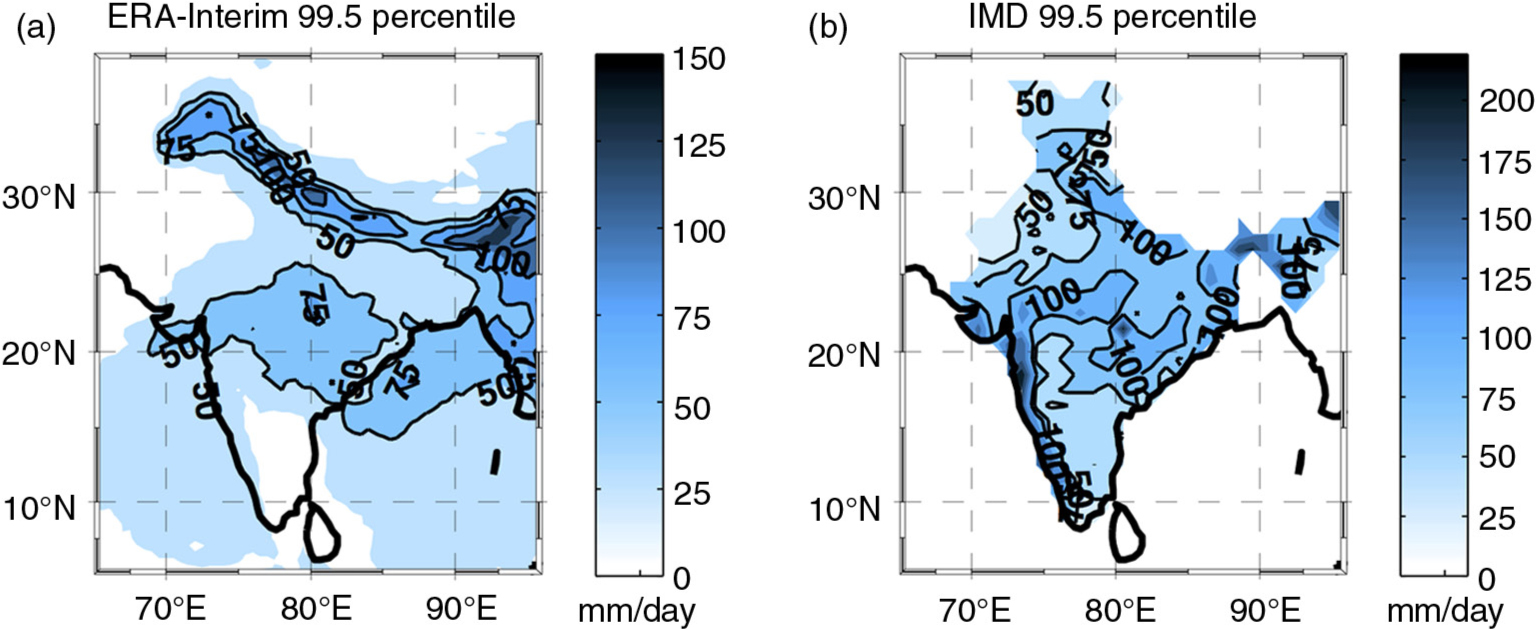
Fig. 2
The 99.5 percentile of daily precipitation calculated for (a) ERA-Interim re-analysis and (b) IMD daily rainfall for the time period 1979–2010. The 50, 75 and 100 mm/d contours are shown in black. Note the different colour bars.
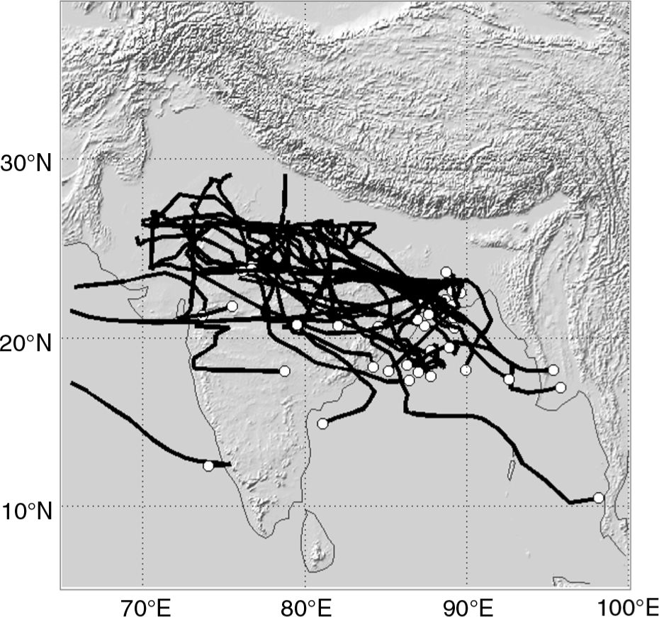
Fig. 3
The LPS trajectories that are related to an extreme rainfall event for the time period 1979–2010, with regard to the different criteria. The white circles indicate the start position of the LPS. The grey shading indicates the topography. See text for a further explanation.
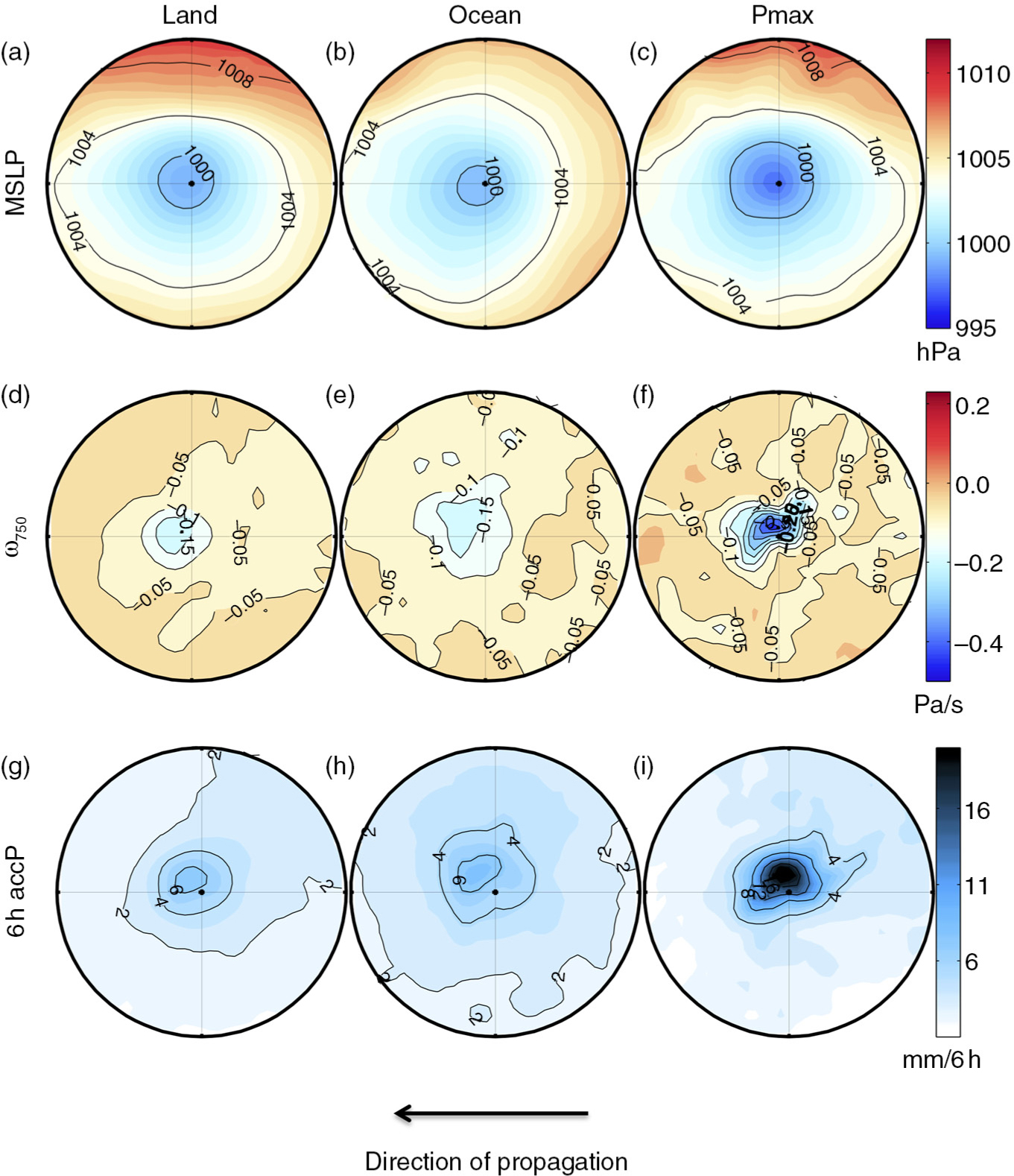
Fig. 4
Composite results of LPS-related MSLP (upper row; a–c), ω 750 (middle row; d–f) and 6 h accumulated precipitation (bottom row; g–i) for the period 1979–2010. The column to the left shows the composite over land, the middle column shows the composite over ocean and the right column shows the composite for the time of maximum precipitation. The direction of movement is from east to west. Note that negative (positive) ω is upward (downward) motions.
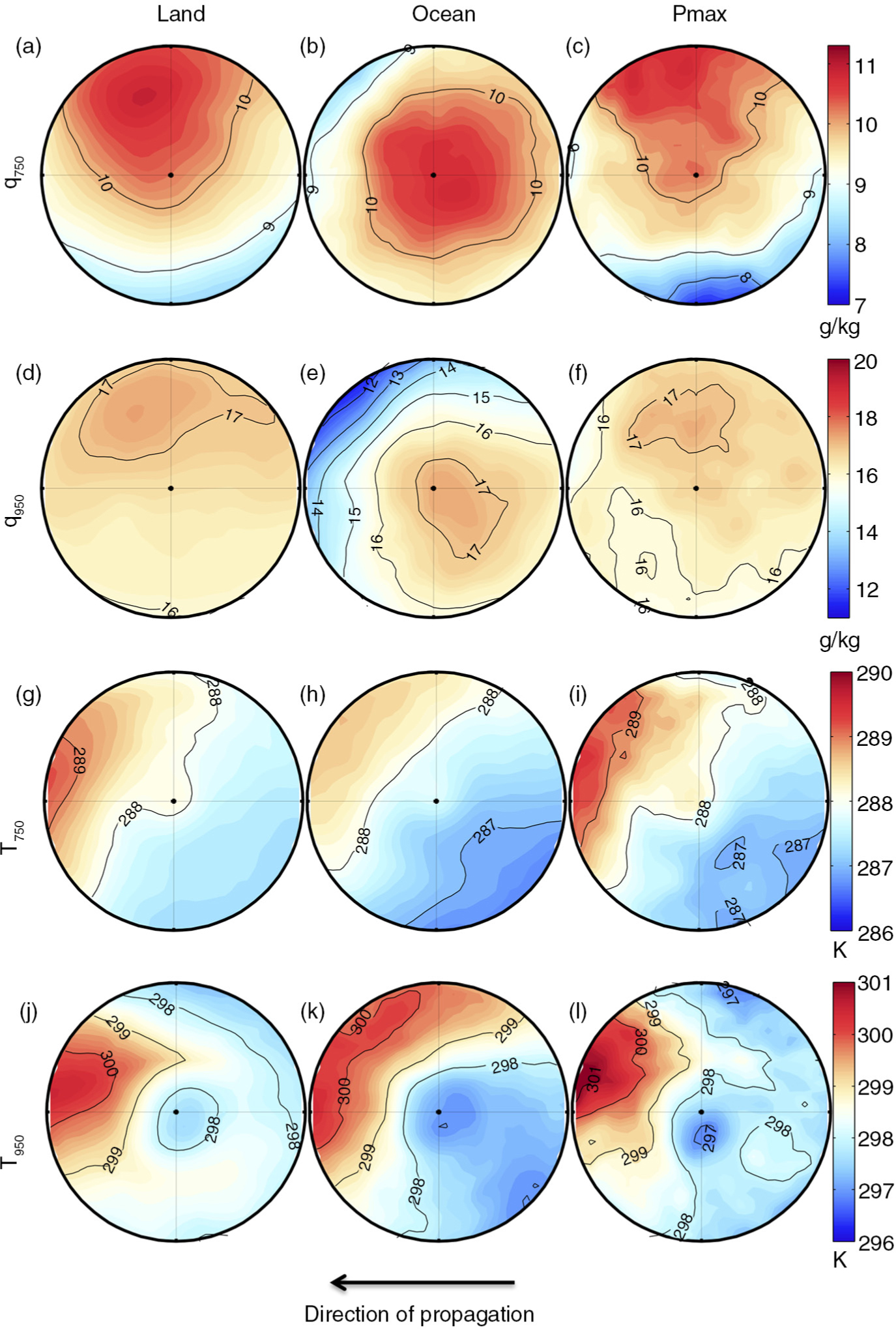
Fig. 5
Same as Fig. 4, but for the parameters q 750 (a–c), q 950 (d–f), T 750 (g–i) and T 950 (j–l).
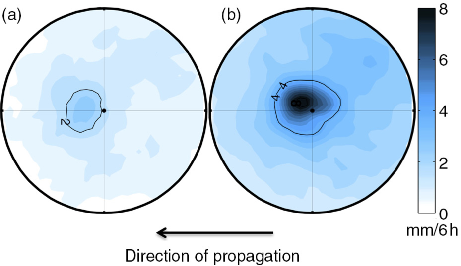
Fig. 6
Comparison of the 6 h accumulated precipitation from TRMM (a) and ERA-Interim (b) for the composite from all time steps.
Table 2. Correlations between the different ERA-Interim parameters (ω 750, T 750, T 950, q 750, q 950, dT/dP) for the different composites: over land, over ocean and Pmax.
ω750Land
Ocean
Pmax 1T750Land
Ocean
Pmax−0.09
0.12
0.07 1T950Land
Ocean
Pmax0.00
0.13
0.130.62
0.44
0.75 1q750Land
Ocean
Pmax−0.35
−0.55
−0.580.13
0.22
0.21−0.07
0.04
0.02 1q950Land
Ocean
Pmax−0.30
−0.53
−0.590.14
0.35
0.32−0.04
0.07
0.090.77
0.77
0.90
0.81 1dT/dpLand
Ocean
Pmax−0.09
−0.04
−0.140.05
0.35
−0.27−0.75
−0.68
−0.840.20
0.14
0.140.17
0.21
0.12 1
Table 3. Correlations between the ERA-Interim precipitation for the different composites (land, ocean and Pmax) with the different meteorological parameters (ω 750, T 750, T 950, q 750, q 950, dT/dP), as well as the predicted precipitation from the multivariable linear regression model.
ω750−0.60−0.78−0.75T7500.03−0.08−0.05T950−0.17−0.20−0.27q7500.440.590.64q9500.380.550.57dT/dp0.240.150.36Predicted P0.660.800.83

Fig. 7
Scatterplots with the best-fit regression line (solid line) between the ERA-Interim precipitation (x-axis) and predicted precipitation calculated with the multivariable linear regression model (y-axis). The composite (a) over land, (b) over ocean and (c) the Pmax. The correlations are given in each sub-figure.
Table 4. Sensitivity tests of the statistical model.
dP/dω750 (%/10%)4.34.55.0dP/dq750 (%/10%)9.310.88.3dP/(dT/dp) (%/K)9.45.914.1
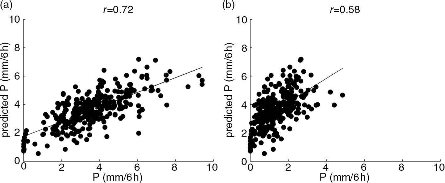
Fig. 8
The predicted precipitation calculated with the predictors from the regression model (y-axis), correlated with ERA-interim precipitation (a) and TRMM precipitation (b) (x-axis). The time period used is 2000–2010.