
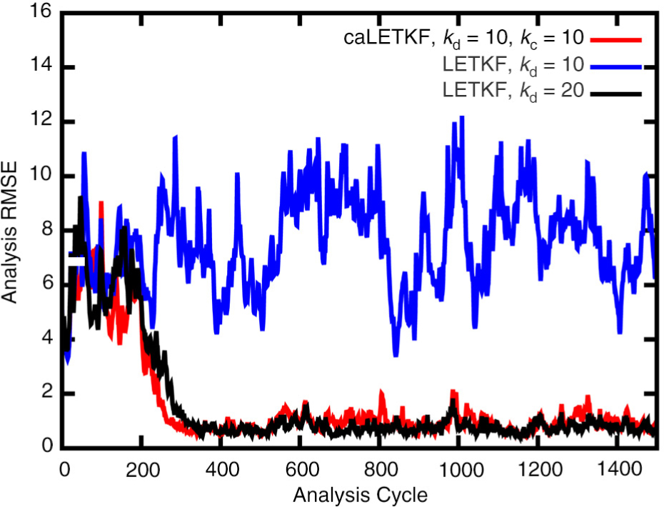
Fig. 1
An example in which a standard LETKF analysis with insufficient ensemble size (10 dynamic ensemble members, blue curve) is stabilised by augmenting the ensemble with 10 additional climatological ensemble members (red curve). The RMS error of the analysis ensemble mean [eq. (6)] is plotted at each analysis cycle over a 1500 analysis cycle period. Both experiments assimilate the same observations on the same observation network. For comparison, results from an experiment where the standard LETKF has k d=20 dynamic ensemble members (black curve) is also included.
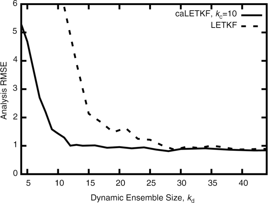
Fig. 2
A comparison of the RMS error of analysis ensemble means, eq. (7), between both the standard LETKF (dashed curve) and the caLETKF (solid curve). After an initial spin-up of 1000 analysis cycles, RMS error is averaged over 50 000 analysis cycles and is plotted as a function of dynamic ensemble size. For the experiments shown here, the climatologically augmented method uses k c=10 climatological ensemble members. Below k d=4 dynamic ensemble members, we find that the caLETKF is susceptible to filter divergence, while the standard LETKF is susceptible to filter divergence below k d=10 dynamic ensemble members.
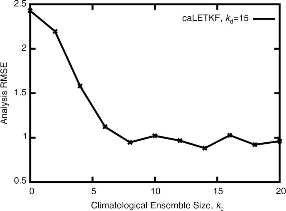
Fig. 3
Here we compare RMS error of the analysis ensemble mean for the caLETKF, eq. (7), as a function of climatological ensemble size k c. Fifteen dynamic ensemble members (k d=15) are used, and each trial is averaged over 50 000 analysis cycles, discarding the first 1000 cycles as spin-up.
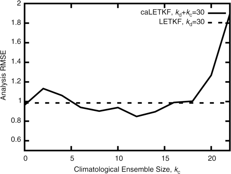
Fig. 4
Analysis accuracy of the caLETKF at constant analysis cost. Here, the sum of the dynamic and climatological ensemble sizes is kept constant at k d+k c=30, and the climatological ensemble size is plotted versus analysis RMS error, eq. (7), averaged over 50 000 analysis cycles, after discarding 1000 initial cycles. For small dynamic ensemble sizes, k d<8 and k c>22, the caLETKF was susceptible to filter divergence.
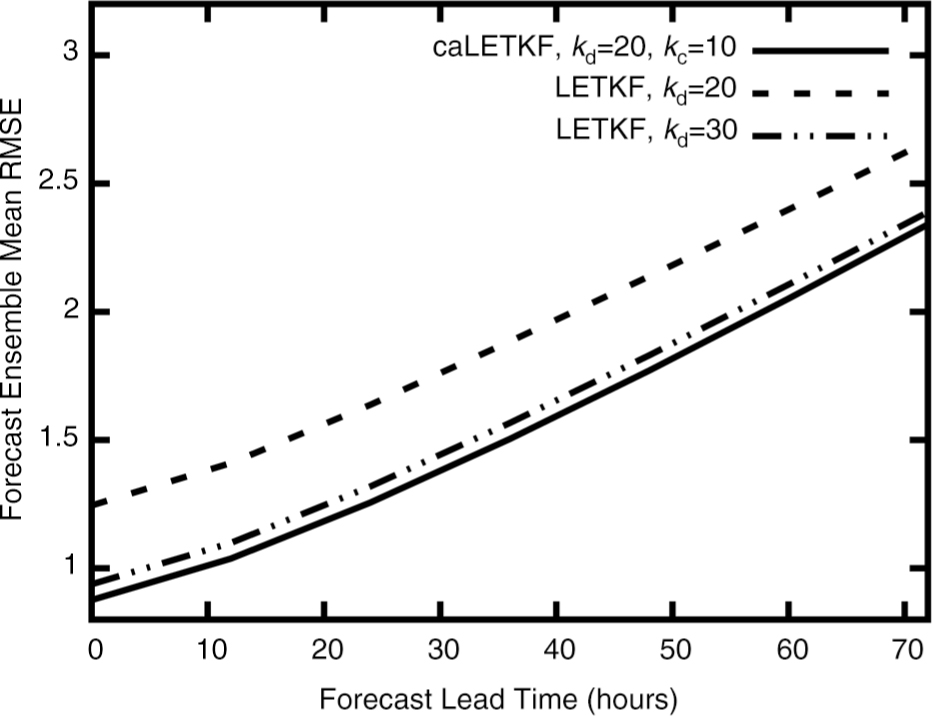
Fig. 5
Ensemble forecast accuracy as a function of lead-time f, for forecasts initialised from caLETKF and LETKF analysis ensembles. Ensembles were forecasted forward in time, and the mean of the forecast ensemble was compared against the truth. The resulting errors were averaged over a sample of 50 000 forecasts at each lead-time, using eq. (7). Forecast results initialised from caLETKF analysis ensembles with k d=20 dynamic and k c=10 climatological ensemble members are shown as a solid black curve. For comparison, results of forecasts initialised from LETKF analysis ensembles with k d=20 and k d=30 dynamic ensemble members are shown as dashed and dot–dashed curves, respectively. The small difference (0.06 in forecast RMSE) between the LETKF k d=30 result and the caLETKF result is within the level of statistical fluctuations seen in our experimental system (for example, see the variation of the solid and dashed curves in Fig. 2 for k d≥30).