
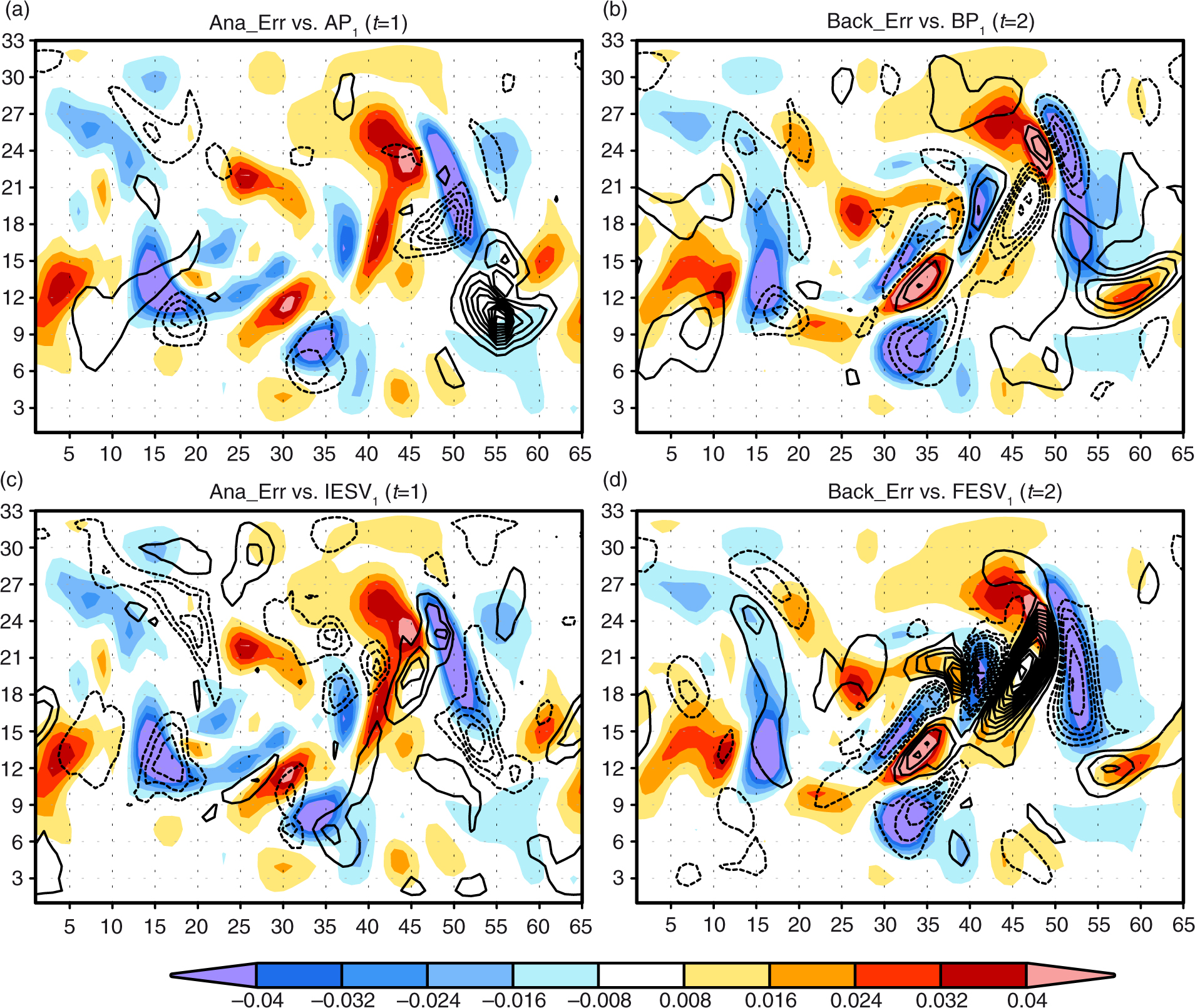
Fig. 1
(a) Analysis ensemble perturbation (contour) and analysis errors (colour shading) at t=1 and (b) and background ensemble perturbation (contour) and background errors (colour shading) at t=2. (c) and (d) are the same as (a) and (b), except that the contours are, IESV1 and FESV1, respectively. The contour interval is 0.004.
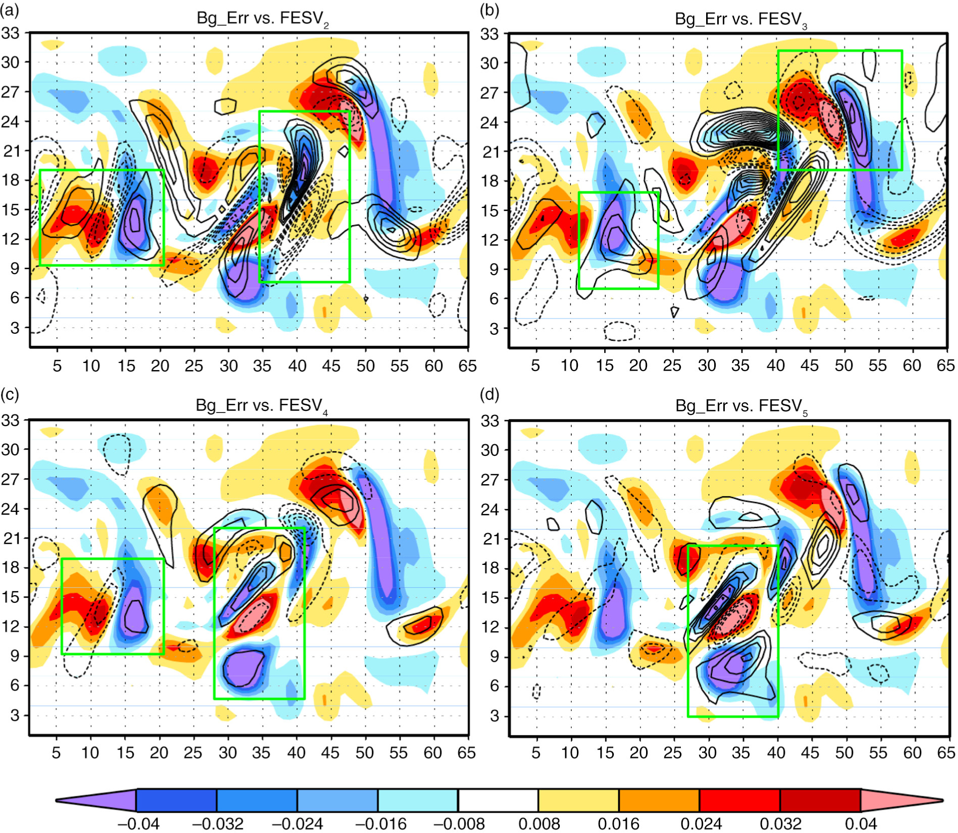
Fig. 2
Background errors (colour shading) and (a) FESV2, (b) FESV3, (c) FESV4 and (d) FESV5 at t=2. Green boxes indicate areas where FESV projects well on the background errors. The contour interval is 0.004.
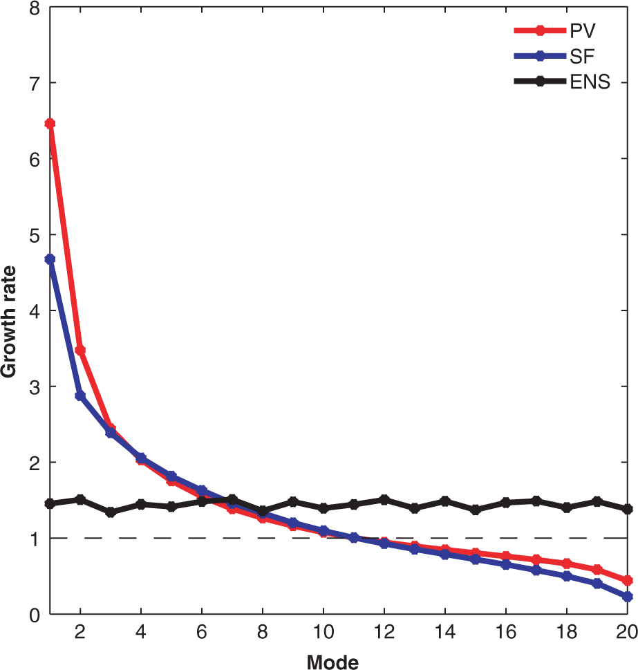
Fig. 3
Time mean growth rates of the 20 ESVs based on the potential vorticity and stream-function norms and ensemble perturbations from 300 analysis cycles. An ESV with a growth rate larger than one indicates a growing mode.
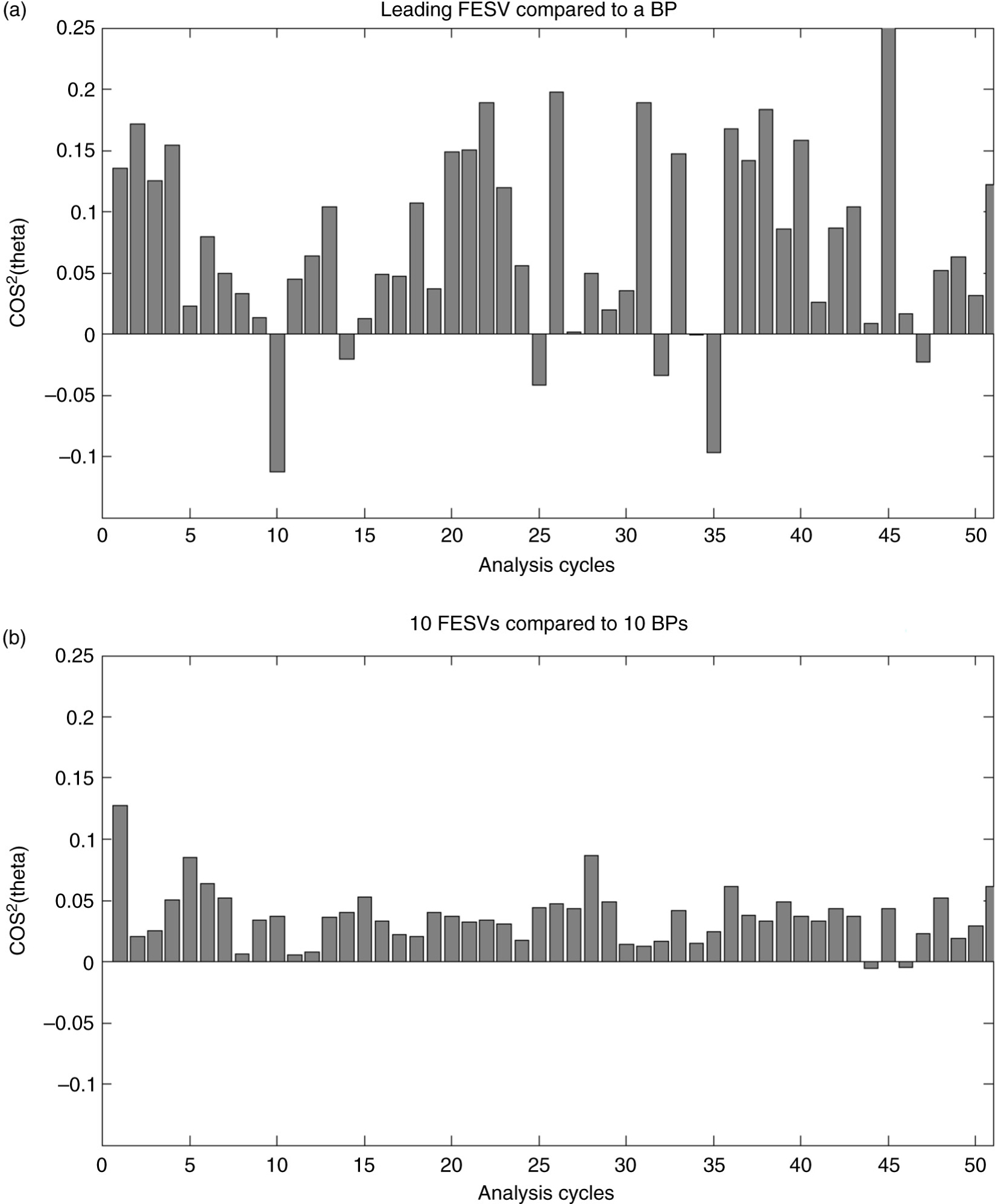
Fig. 4
Time series of the improvement of the projection of the background errors on the FESVs compared with the BPs. (a) leading FESV compared with a BP and (b) 10 FESVs compared with 10 BPs.
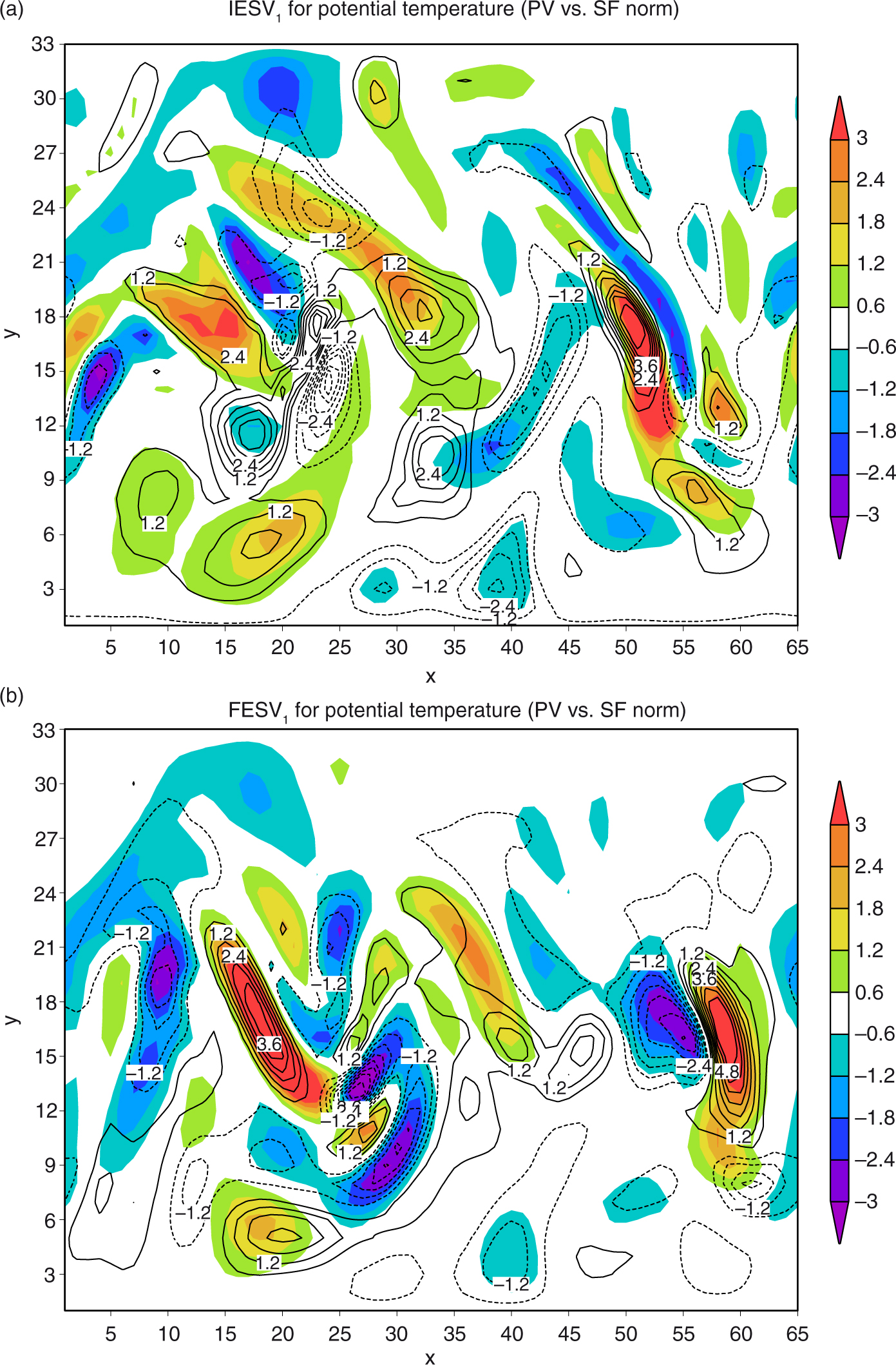
Fig. 5
(a) IESV1 and (b) FESV1 at t=50, derived with the potential vorticity norm (colour shading) and stream-function (contours) norms. For plotting purpose, variables are rescaled and the contour interval is 0.6.
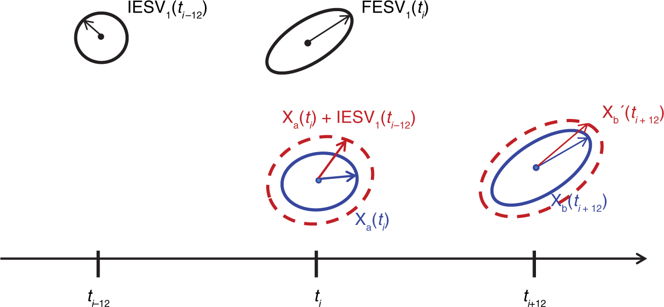
Fig. 6
A schematic plot for applying IESVs as the additive inflation in the LETKF assimilation framework.
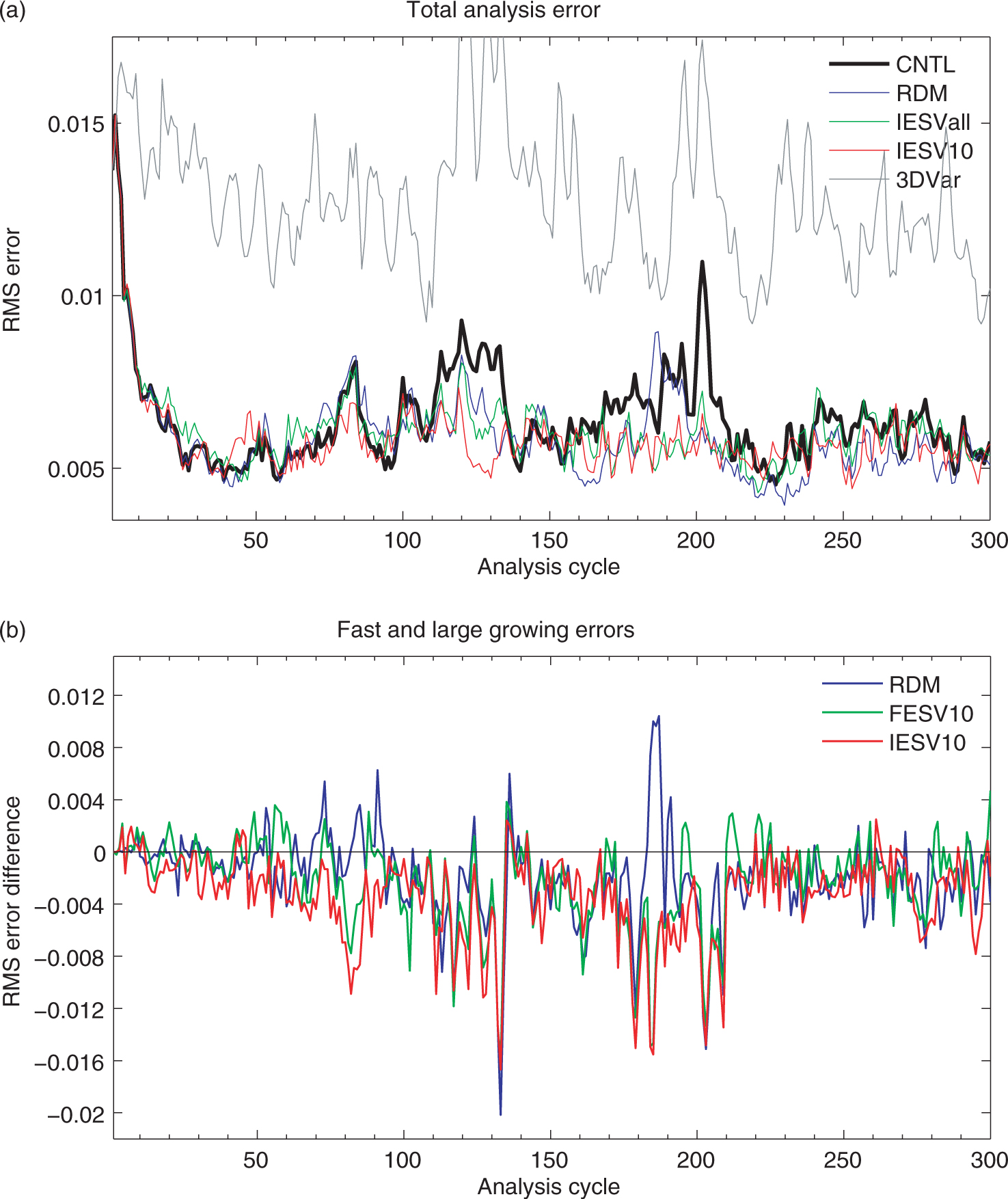
Fig. 7
Time series of the RMS of (a) the total analysis error and (b) analysis error with the mask of large errors. A mask of large errors is defined as the grid points whose analysis error from the CNTL experiment is two standard deviation larger than the domain-average analysis error.
Table 1. Time mean analysis and background errors of all experiments
RMSE (analysis/background)6.4 (7.5)5.8 (6.7)5.9 (6.8)5.6 (6.4)6.3 (7.2)5.9 (6.9)6.5 (7.4)RMSE_Large (analysis/background)13.0 (18.3)10.8 (14.8)9.7 (13.4)9.1 (12.2)9.9 (13.8)10.3 (14.4)10.7 (14.8)
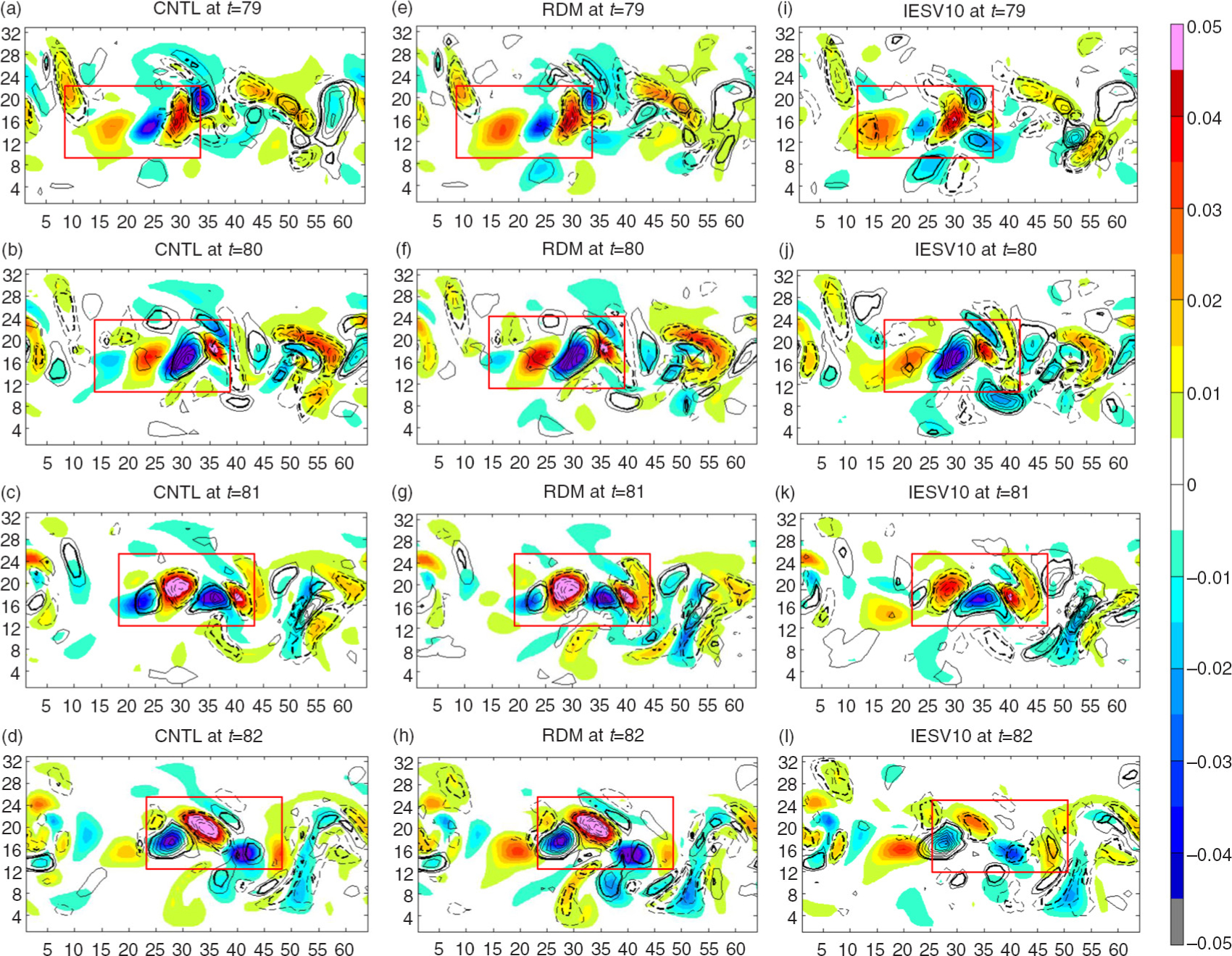
Fig. 8
(a)–(d) Background error (shading) and analysis increment (contour, black: positive, grey: negative) of potential temperature at the bottom level from the CNTL experiment from t = 79 to t = 82. Figure 8(e)–(h) are the same as Fig. 8(a)–(d) except that they are derived from the RDM experiment. Figure 8(i)–(k) are the same as Fig. 8(a)–(d) except that they are derived from the IESV10 experiment. The contour interval is 0.005, and the solid and dashed thick lines denote iso-lines of 0.005 and −0.005, respectively.
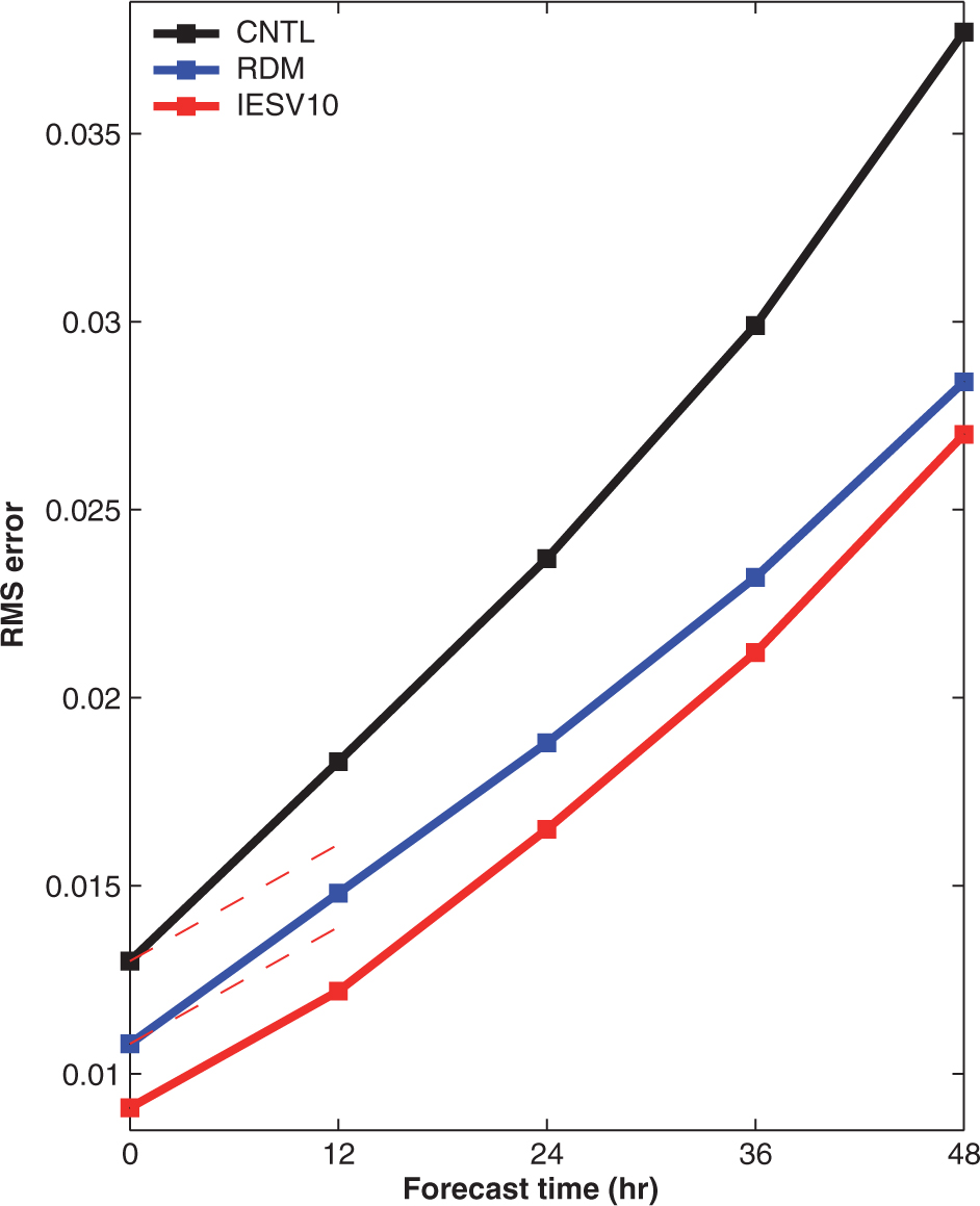
Fig. 9
Time mean RMS analysis/forecast errors at different forecast lead times with the mask of large errors. The red dashed line is the error of IESV10.
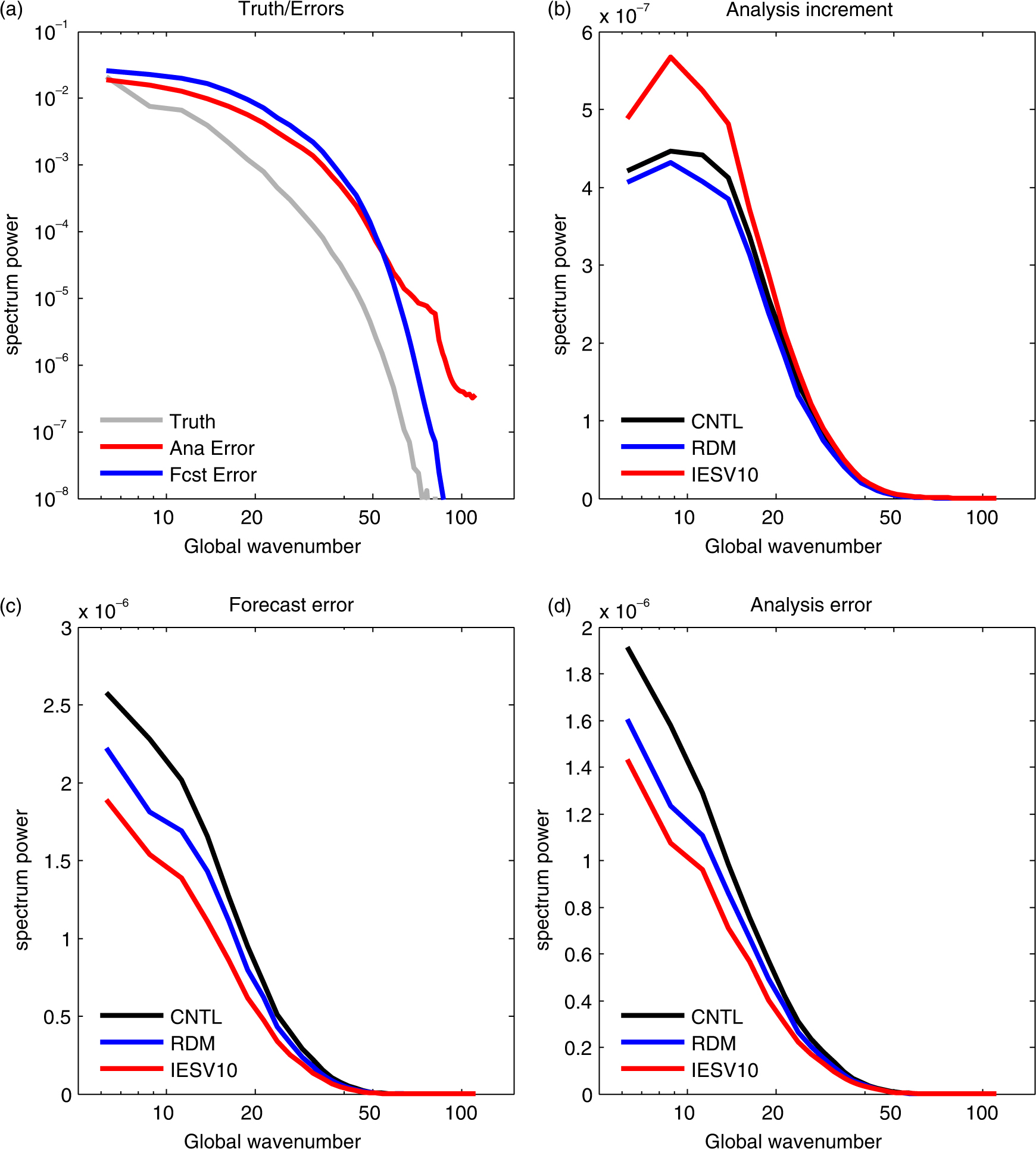
Fig. 10
Spectrum power of (a) truth, forecast and analysis errors of CNTL, (b) analysis increments from CNTL, RDM and IESV10 (c) same as (b) except for the forecast error and (d) same as (b) except for the analysis error. The amplitude of the spectrum power of analysis and forecast errors is multiplied in Fig. 9a by a constant factor, 104, for plotting purposes.
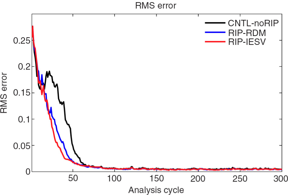
Fig. 11
Time series of the RMS analysis error of the potential temperature at the bottom level.
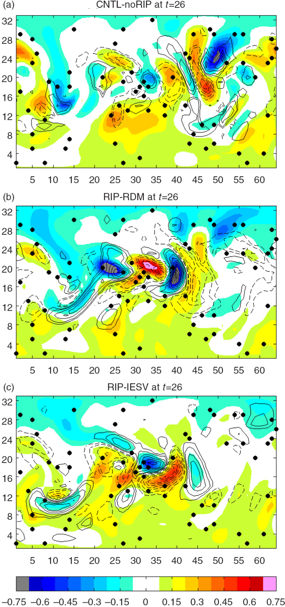
Fig. 12
Analysis increment (contours) and background error (colour shading) of the potential temperature at the bottom level at t=26 from (a) CNTL-noRIP, (b) RIP-RDM and (c) RIP-IESV. For Fig. 12, the scale is twice as shown. The contour interval is 0.075.