
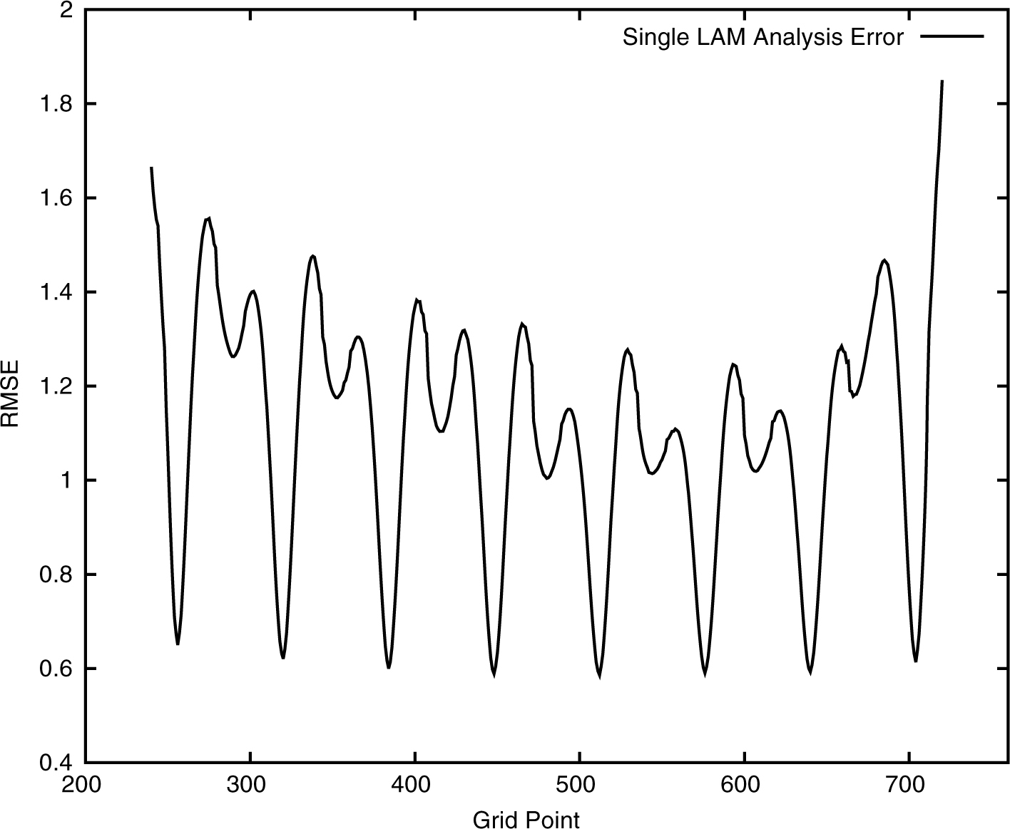
Fig. 1
RMS analysis errors of the ensemble mean when the LETKF is performed using only the state information of a single LAM. The LAM is defined over grid points [240,720]. The RMS errors shown are averaged over 2×10⁴ analysis cycles. Boundary condition errors can be seen in the increase in RMS error at grid points near the LAM boundary.
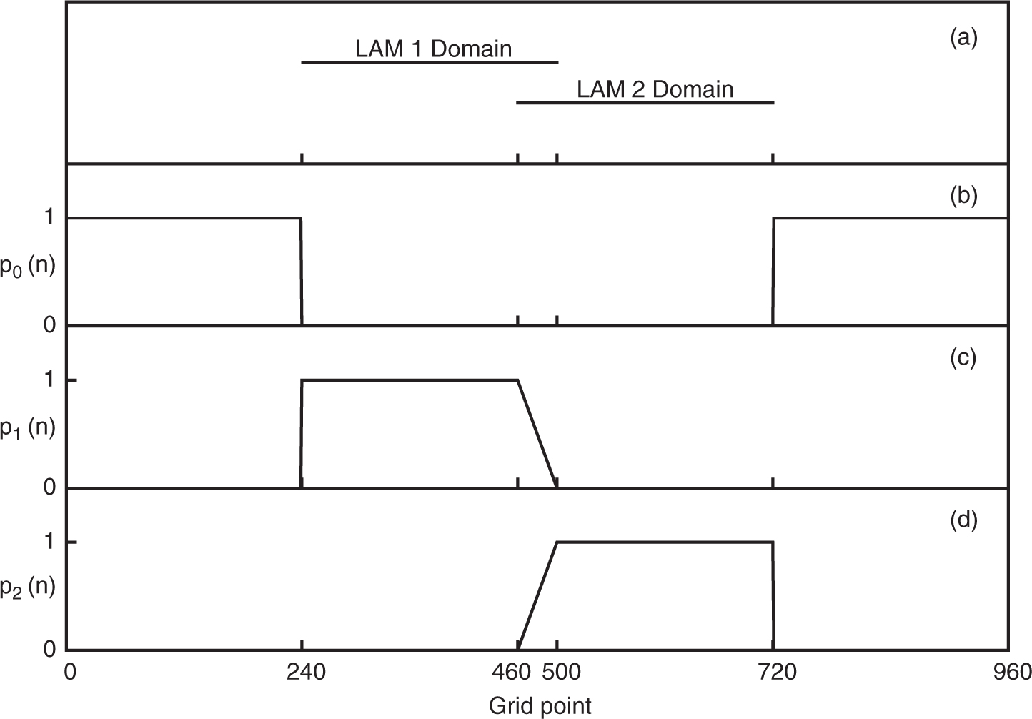
Fig. 2
An example of the p i functions for a scenario with two limited-area models, denoted LAM 1 and LAM 2, used in one of our experiments. Part (a) shows the domains on which the LAMs are defined, which cover grid point intervals of [240,500] and [460,720]. Parts (b)–(d) show the functional form of the p i functions for the global model, p 0 (n) [shown in panel (b)], and each of the limited-area models,p 1 (n) and p 2 (n) [shown in panels (c) and (d), respectively]. All plots show grid point location n on the horizontal axis.
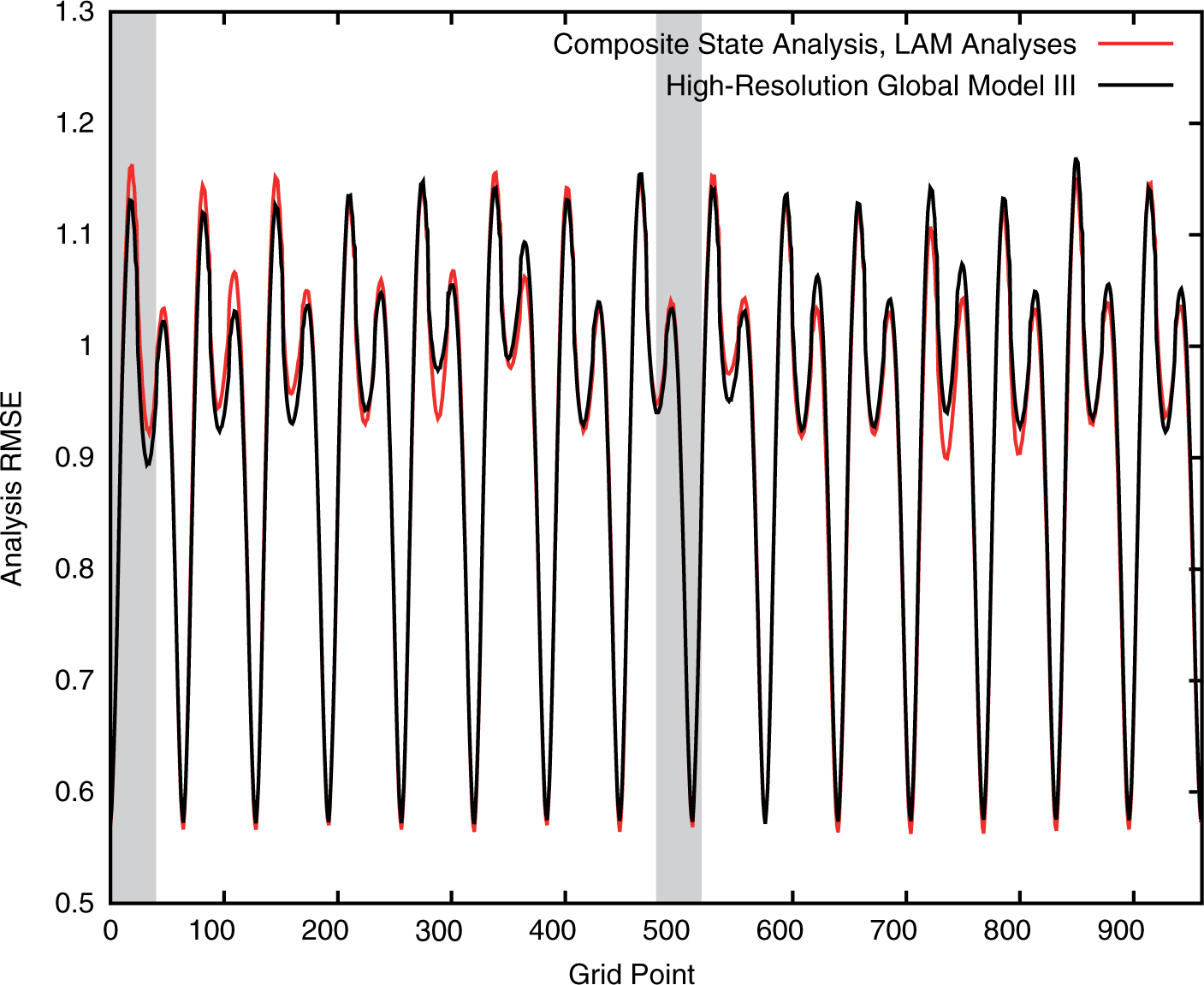
Fig. 3
RMS analysis errors of the composite state ensemble mean (red curve). For comparison, the analysis error of the ensemble mean for a global high-resolution perfect model LETKF analysis (black curve) is also shown. LAMs are defined over grid points [0,520] and [480,40], and statistics are taken over 105 analysis cycles, discarding the first 103 cycles. The shaded areas indicate the domain where both LAMs are defined.
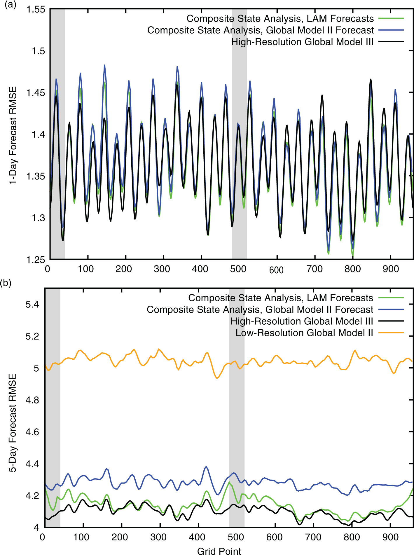
Fig. 4
(a) RMS 1-d and (b) 5-d forecast errors, initialised using the composite state analysis ensemble mean. The green curves in both panels show errors of forecasts produced by the LAMs, while the blue curves show errors for forecasts produced by the low-resolution, imperfect global model. For comparison, forecast errors produced by a global high-resolution perfect model and a global low-resolution imperfect model, initialised from an LETKF analysis are shown as black curves [in panels (a) and (b)] and an orange curve [in panel (b)], respectively. Both panels show results using the conditions described in Fig. 3, and the shaded areas indicate regions of LAM domain overlap.

Fig. 5
RMS analysis and 1-d forecast errors of the global model ensemble mean, averaged over all grid points and time (105 analysis cycles), discarding 103 initial spin-up cycles, and performing the analysis using the composite state method. The results shown above are for two LAMs whose domains tile the globe. The x-axis shows the number of grid points that the LAM domains have in common. For these models, there appears to be no benefit to large LAM domain overlap.

Fig. 6
RMS 1-d forecast errors, averaged over 105 analysis cycles, in the ‘Large World’ scenario. The experimental domain runs from n=0 to 1920, and LAMs are defined over grid point intervals [0,540], [480,1020], [960,1500] and [1440,60]. The blue curve shows forecasts, initialised using the composite state analysis ensemble mean, made with the low-resolution global model. Observations are located at every 64 grid points, and the shaded areas indicate grid point intervals where more than one LAM domain is defined.

Fig. 7
RMS analysis errors of the ensemble mean and 1-d forecast errors calculated using the composite state method, when the entire simulation domain is divided amongst different numbers of LAM domains. In a given experiment, each of the LAM domains are the same size, so that the LAM domains are 521 grid points long in the two LAM case, 261 grid points long in the four LAM case, 131 grid points long in the eight LAM case, and 65 grid points long in the 16 LAM case. Errors begin to increase as the area influenced by boundary condition errors becomes a larger part of the total LAM domain. Statistics are averaged first over 105 analysis cycles, discarding the first 103 cycles, then over all grid points.
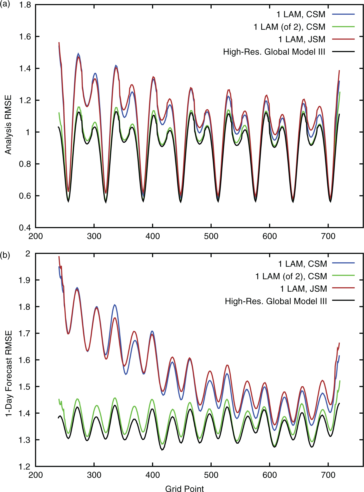
Fig. 8
(a) Ensemble mean analysis and (b) 1-d forecast accuracy gains with the addition of a second LAM. Statistics are gathered over 105 analysis cycles, after 103 cycles of spin-up time. In both the one and two LAM situations the LAM domain of interest runs from grid points [240,720]. The second LAM is added on the domain [720,240]. Curves denoted ‘CSM’ are calculated using the composite state method, and those denoted ‘JSM’ are found when using the joint-state method of Yoon et al. (2012). Single deterministic forecasts are initialised with the LAM analysis ensemble mean. The results from the perfect model ensemble are included over the LAM domain of interest as a benchmark for comparison.

Fig. 9
Ensemble mean forecast accuracy of the global model, for the conditions described for Fig. 8. The addition of a second LAM dramatically lowers global model forecast accuracy over the entire global domain. Results from perfect and imperfect global model ensemble forecasts are included as a benchmark for comparison, and vertical black lines demarcate the LAM boundaries.
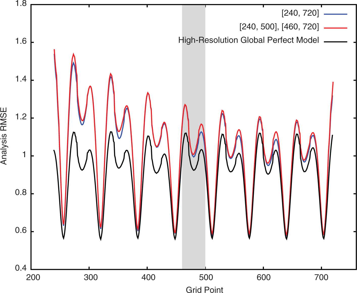
Fig. 10
RMS analysis errors of the ensemble mean calculated using the composite state method for two model scenarios. The first scenario has a single LAM defined over the grid point interval [240,720] (blue curve), and the second has two LAMs defined over the intervals [240,500] and [460,720] (red curve). The analysis error of the ensemble mean of a global high-resolution perfect model LETKF (black curve) is included as a benchmark for comparison. Statistics are gathered over 105 analysis cycles, discarding the first 103 cycles. The shaded area indicates the domain where both LAMs are defined.