
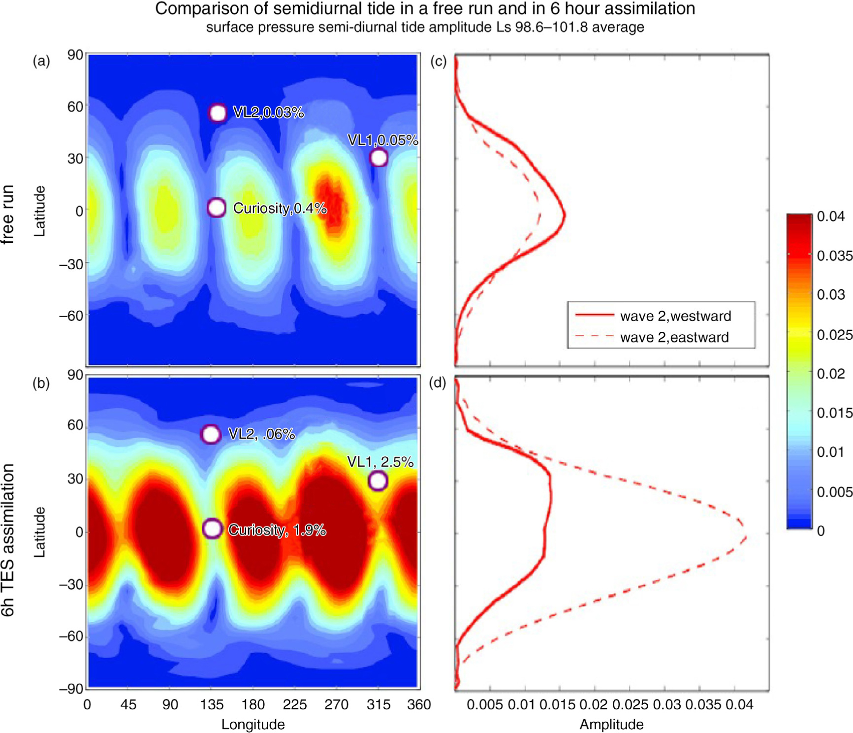
Fig. 1
Surface pressure semi-diurnal tide amplitude spatial distribution (a, b) and wave 2 amplitude (c, d). (a) and (c) are from free runs, and (b) and (d) are from 6-hr TES assimilation: all are with ice cloud parameterisation. ‘Wave 2, westward’ corresponds to A2,2/migrating tide, and ‘wave 2, eastward’ to A-2,2/non-migrating tide/SE2. Viking Lander and Curiosity sites location and their corresponding tides amplitudes from model simulations are shown in (a, b). All amplitudes are a percentage of the diurnally averaged surface pressure.
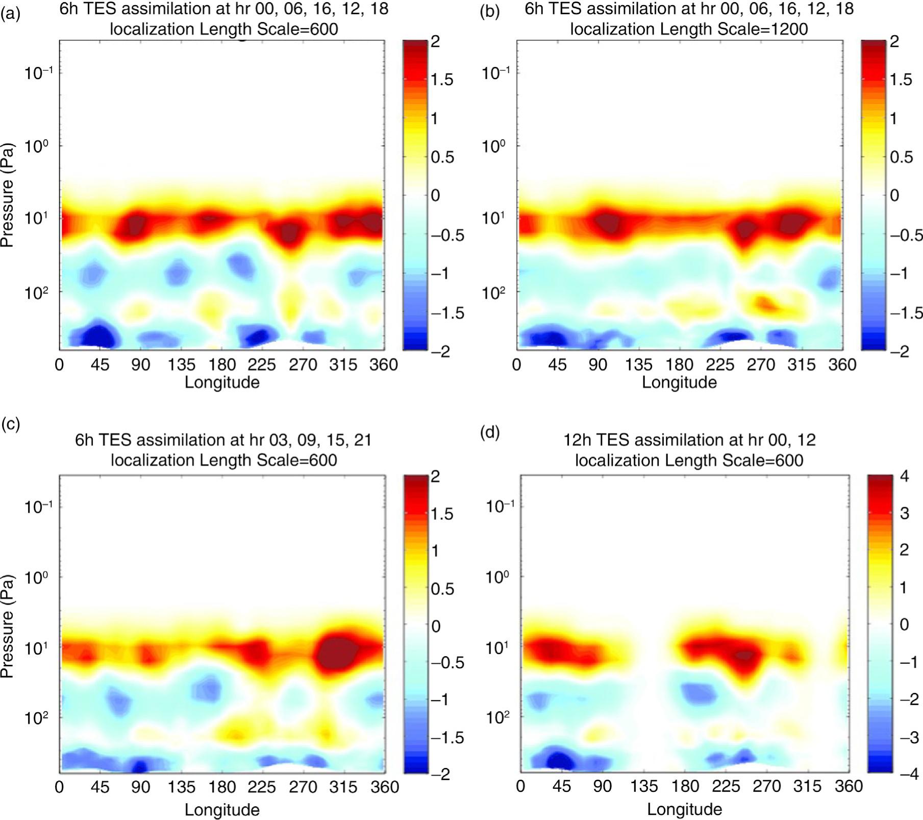
Fig. 2
Equatorial daily average temperature analysis increment for different assimilations. (a) represents the original 6-hr TES assimilation assimilating observation at hour 00, 06, 12 and 18 with localisation length scale=600; (b) is the same as (a), but with doubled localisation length scale; (c) is the same as (a), but assimilates observation at hour 03, 09, 15 and 21; (d) is the 12-hr TES assimilation assimilating observation at hour 00 and 12 with localisation length scale=600. All are with ice cloud parameterisation.
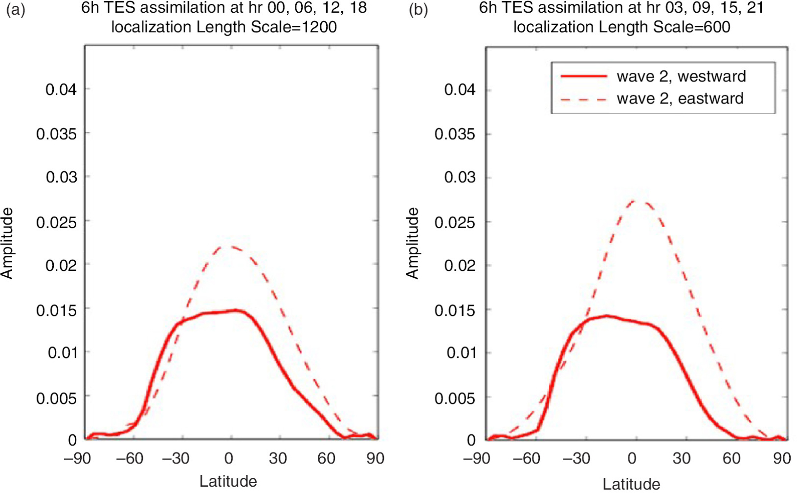
Fig. 3
Surface pressure semi-diurnal tide wave 2 amplitude for TES assimilations. (a) is the 6-hr TES assimilation updating observation at hour 00, 06, 12 and 18 with a doubled localisation length scale = 1200, (b) is the 6-hr TES assimilation updating observation at hour 03, 09, 15 and 21 with a localisation length scale = 600. Both are with ice cloud parameterisation. Compare to Fig. 1d. As in Fig. 1, ‘wave 2, westward’ corresponds to A2,2/migrating tide, and ‘wave 2, eastward’ to A-2,2/non-migrating tide/SE2.

Fig. 4
Surface pressure diurnal tide amplitude spatial distribution (a–c) and wave 1 amplitude (d–f). (a) and (d) are from free runs, (b) and (e) are from 6-hr TES assimilation and (c) and (f) are from 12-hr TES assimilation: all are with ice cloud parameterisation. ‘Wave 1, westward’ corresponds to A1,1/migrating tide, and ‘wave 1, eastward’ to A-1,1/non-migrating tide/DE1.

Fig. 5
Schematic illustration of the 6-hr 3D-LETKF, 6-hr 4D-LETKF, 2-hr 3D-LETKF, 2-hr 4D-LETKF and 1-hr 3D-LETKF Panel (b) is from Greybush et al. (2012). In 4D-LETKF, observations (combined together as red/pink line segments to discern between different time slots) are compared to forecasts (solid blue lines) at their correct hours rather than just to the 6-hr/2-hr/1-hr forecast as in the 3D-LETKF.
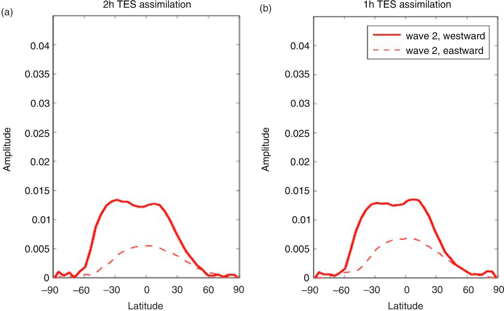
Fig. 6
Surface pressure semi-diurnal tide wave 2 amplitude for TES assimilations. (a) is 2-hr LETKF assimilation, and (b) is 1-hr LETKF assimilation. Both are with ice cloud parameterisation. Compare to Fig. 1d. As in Fig. 1, ‘wave 2, westward’ corresponds to A2,2/migrating tide, and ‘wave 2, eastward’ to A-2,2/non-migrating tide/SE2.

Fig. 7
Seven-day composite daily average surface pressure bias (a–c) and level 10 (50 Pa) temperature bias (d–e) over sol 397–403 (L s 98.6°–101.7°) for 6-hr (a, d), 2-hr (b, e) and 1-hr (c, f) of TES assimilation. All are with ice cloud parameterisation.
Table 1. Surface pressure diurnal and semi-diurnal tide amplitudes at Viking Lander and Curiosity sites; all are shown in percentages relative to the diurnal average surface pressure
Obs
(%)free run LETKF
(%)TES 6-hr LETKF
(%)TES 2-hr LETKF
(%)TES 1-hr LETKF
(%) Obs
(%)free run
(%)TES 6-hr LETKF
(%)TES 2-hr LETKF
(%)TES 1-hr LETKF
(%)
VL1~12.21.31.61.60.3–0.40.052.50.30.5VL2NA1.00.70.80.9NA0.030.60.20.2Curiosity3.43.83.33.13.20.5–0.60.41.90.90.9
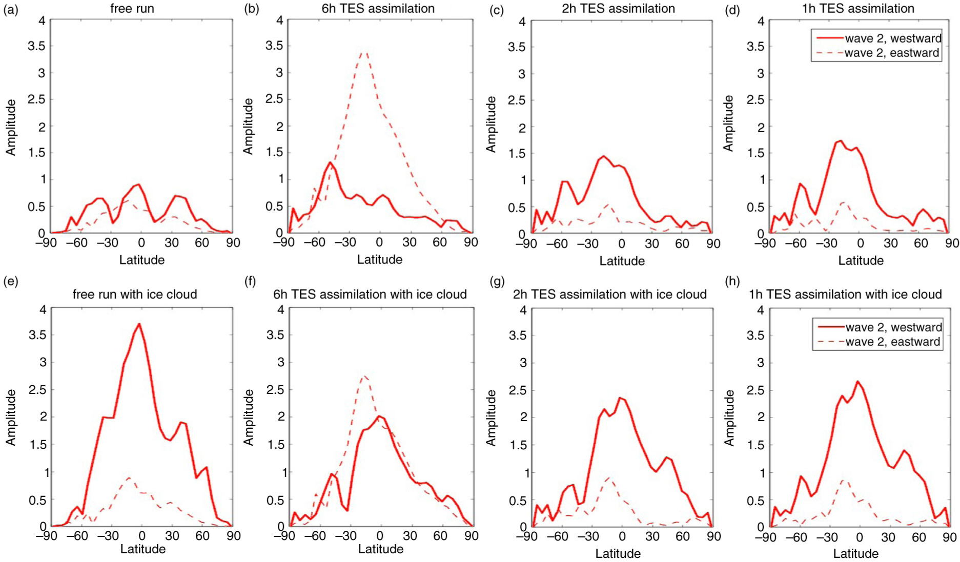
Fig. 8
50 Pa temperature semi-diurnal tide wave 2 amplitude for free run and TES assimilations. (a) and (e) are from free run; (b–d) and (f–h) are from TES assimilations, 6, 2 and 1, respectively. (a–d) are without ice cloud parameterisation, and (e–f) are with ice cloud parameterisation. As in Fig. 1, ‘wave 2, westward’ corresponds to A2,2/migrating tide, and ‘wave 2, eastward’ to A-2,2/non-migrating tide/SE2.
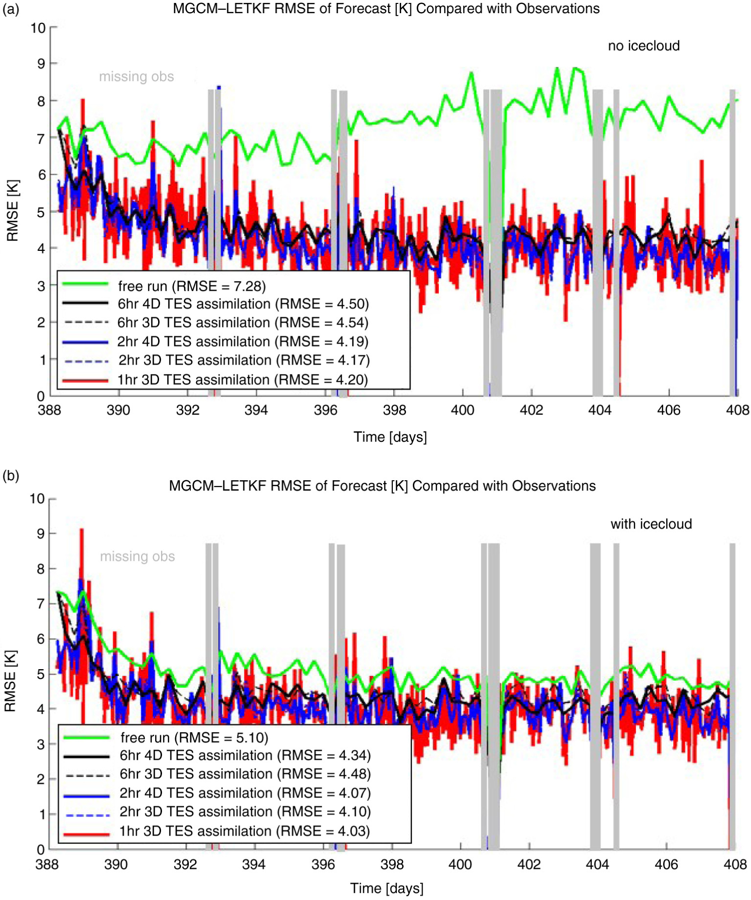
Fig. 9
Performance of the MGCM-LETKF and the free run (without assimilating observation) during NH summer (~Ls 100), evaluated by comparing RMSD of the background forecasts from TES observations. (a) is without ice cloud parameterisation and (b) is with ice cloud parameterisation. Time slots without observation are shaded in grey. Time-averaged RMS difference is denoted in the legend.
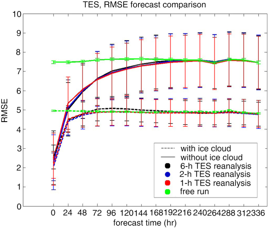
Fig. 10
Performance of the MGCM-LETKF during NH summer (~Ls 100), evaluated by comparing RMS differences of forecasts based on hour 00 and hour 12 forecasts from TES assimilations with TES observations, without and with ice cloud parameterisation. Error bar with one standard deviation for each experimental run is also included.
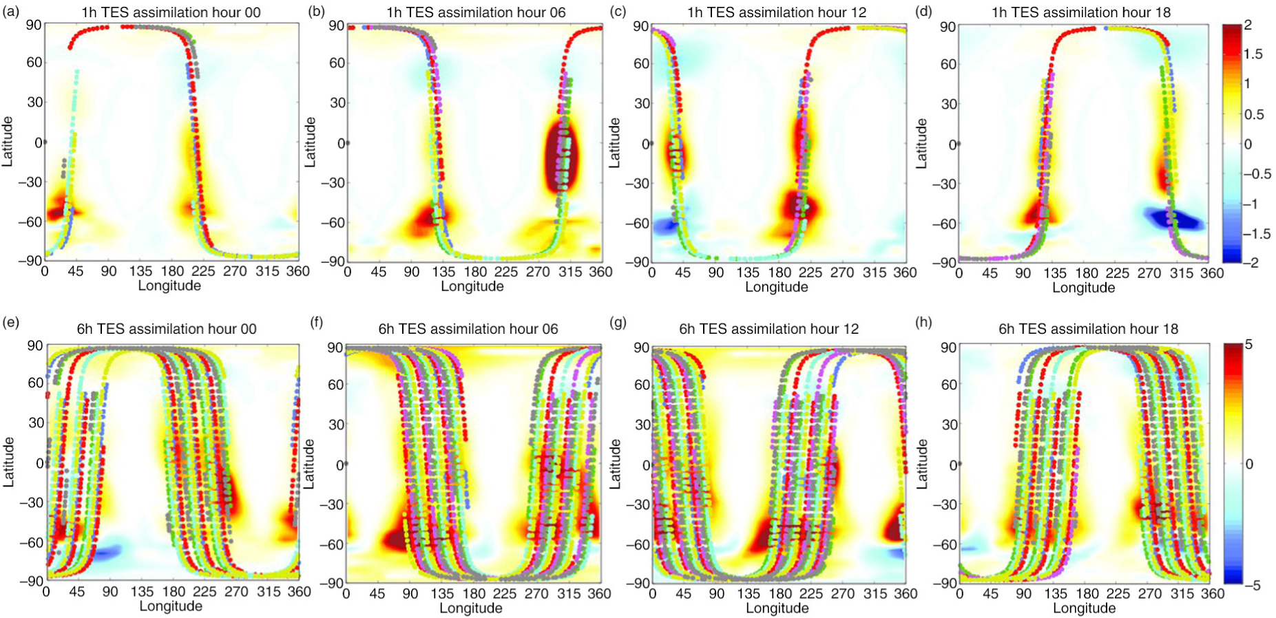
Fig. 11
Seven-day composite bias pattern (shaded colours) and observation track (dots) over sol 397–403 (L s 98.6°–101.7°) at level 10 for 6-hr TES assimilation (a–d), and 1-hr TES assimilation (e–h), at different times a day: hour 00 (a), (e); hour 06 (b), (f); hour 12 (c), (g); and hour 18 (d), (h). Different colours of dots represent observation path at different day. All are without ice cloud parameterisation.
Table 2. Time-averaged RMSD of the 6-hr and1-hr MGCM-LETKF TES reanalysis during NH summer (~Ls 100), without and with bias correction (both sliding window daily average bias correction and sliding window diurnal bias correction), without radiatively active water ice cloud (RAC) parameterisation
no Bias Correction (BC)
without RAC6-hr TES assimilation
Daily-ave BC
without RAC6-hr TES assimilation
Diurnal BC
without RAC6-hr TES assimilation
no BC
with RAC
RMSD4.504.143.964.34Experimental run1-hr TES assimilation
no BC
without RAC1-hr TES assimilation
Daily-ave BC
without RAC1-hr TES assimilation
Diurnal BC
without RAC1-hr TES assimilation
no BC
with RACRMSD4.203.863.784.03
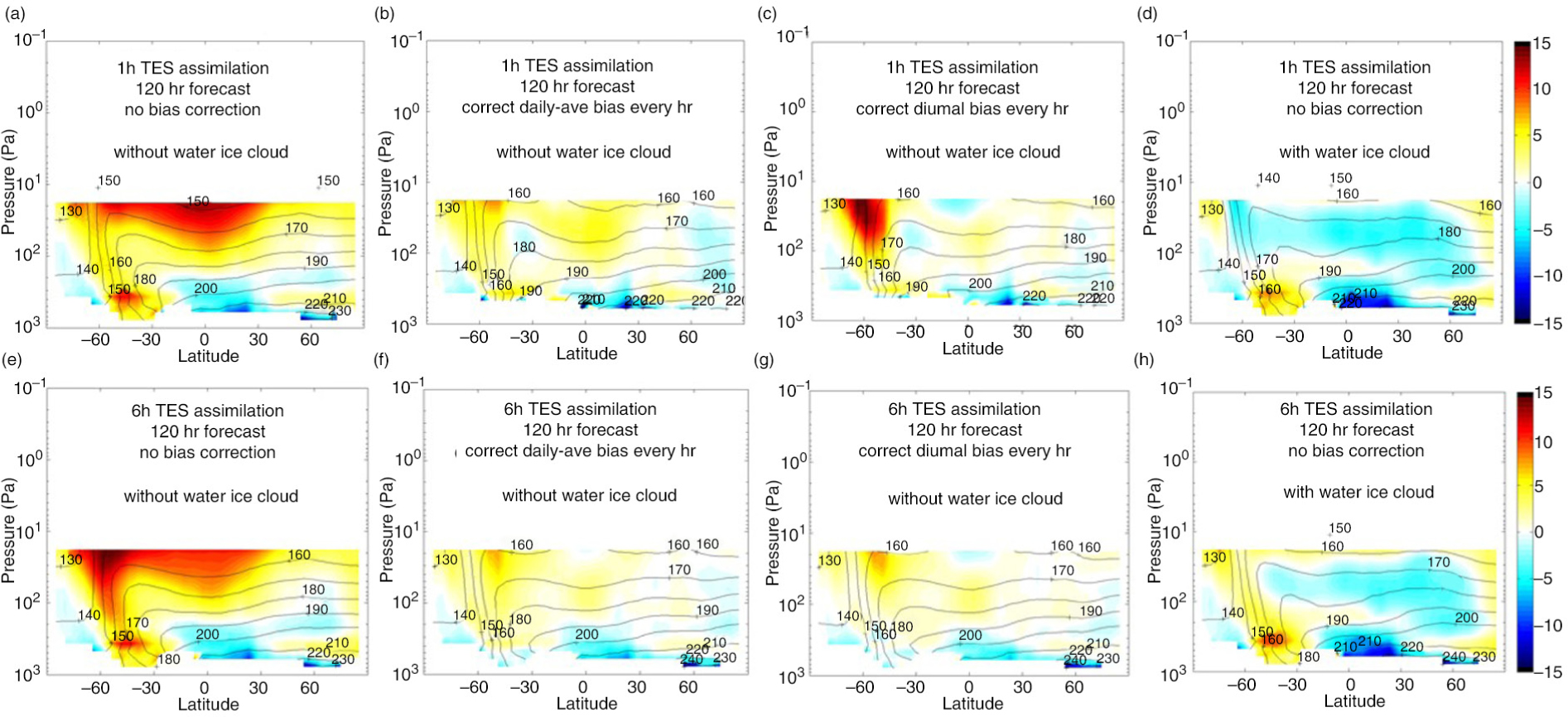
Fig. 12
Bias pattern of 120-hr forecast in 1-hr TES LETKF (a–d) and 6-hr TES LETKF (e–h) runs. Left panels are original forecast without bias correction; second column panels correct the sliding window daily average bias every 1 hr/6 hr; third column panels correct the sliding window diurnal bias every 1 hr/6 hr; the above-mentioned panels are all without RAC parameterisation; right panels are original forecast without bias correction, but with RAC parameterisation.