
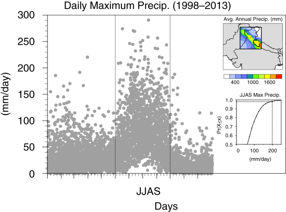
Fig. 1
Daily maximum precipitation for the NW subset of India (see inset) from 1998 to 2013. The time-series for each year are overlaid. The inset map also shows the average annual accumulated precipitation for this region (1998–2013). The Uttarakhand state is highlighted with thicker boundary lines in the inset map. Also, shown is the Cumulative Distribution Function [CDF, Pr(X≤x)] of the daily maximum rainfall for JJAS (1998–2013). The exceedance probability of 200 mm/d was estimated as 1.6%.
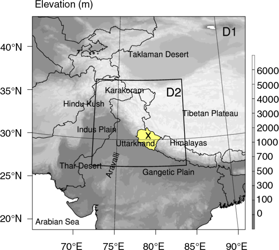
Fig. 2
Model domain and orography (m) with relevant geographical features. D1 and D2 have horizontal model resolutions of 7 km and 2.8 km respectively. The Ukhimath station in Uttarakhand state (masked in yellow), where the flood event took place is marked with X (30.30°N, 79.25°E).
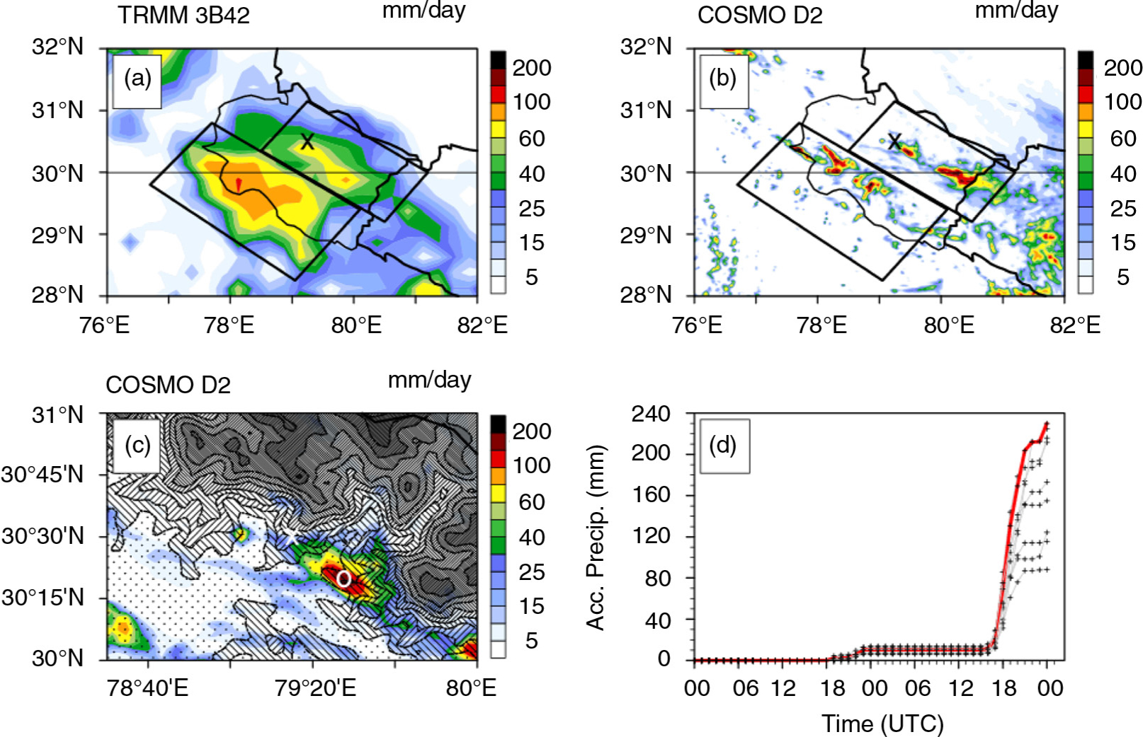
Fig. 3
(a) Daily accumulated precipitation on 13 September 2012 from TRMM 3B42 data; (b) Daily accumulated precipitation on 13 September 2012 simulated using COSMO (D2 domain). Two bands of precipitation are outlined by frames [in (a) and (b)] along with the borders of Uttarakhand state. (c) Zoomed modelled accumulated precipitation with the local topography at the resolution of the D2 model domain (2.8 km). The topography contour interval is 500 m reaching from 2000 to 6000 m elevation. (d) Time-series of accumulated precipitation at location marked ‘o’ (red) and the surrounding grid cells (grey), starting 12 September 2012. The precipitation accumulation shown in the spatial distributions is derived from 0000 UTC to 2330 UTC.
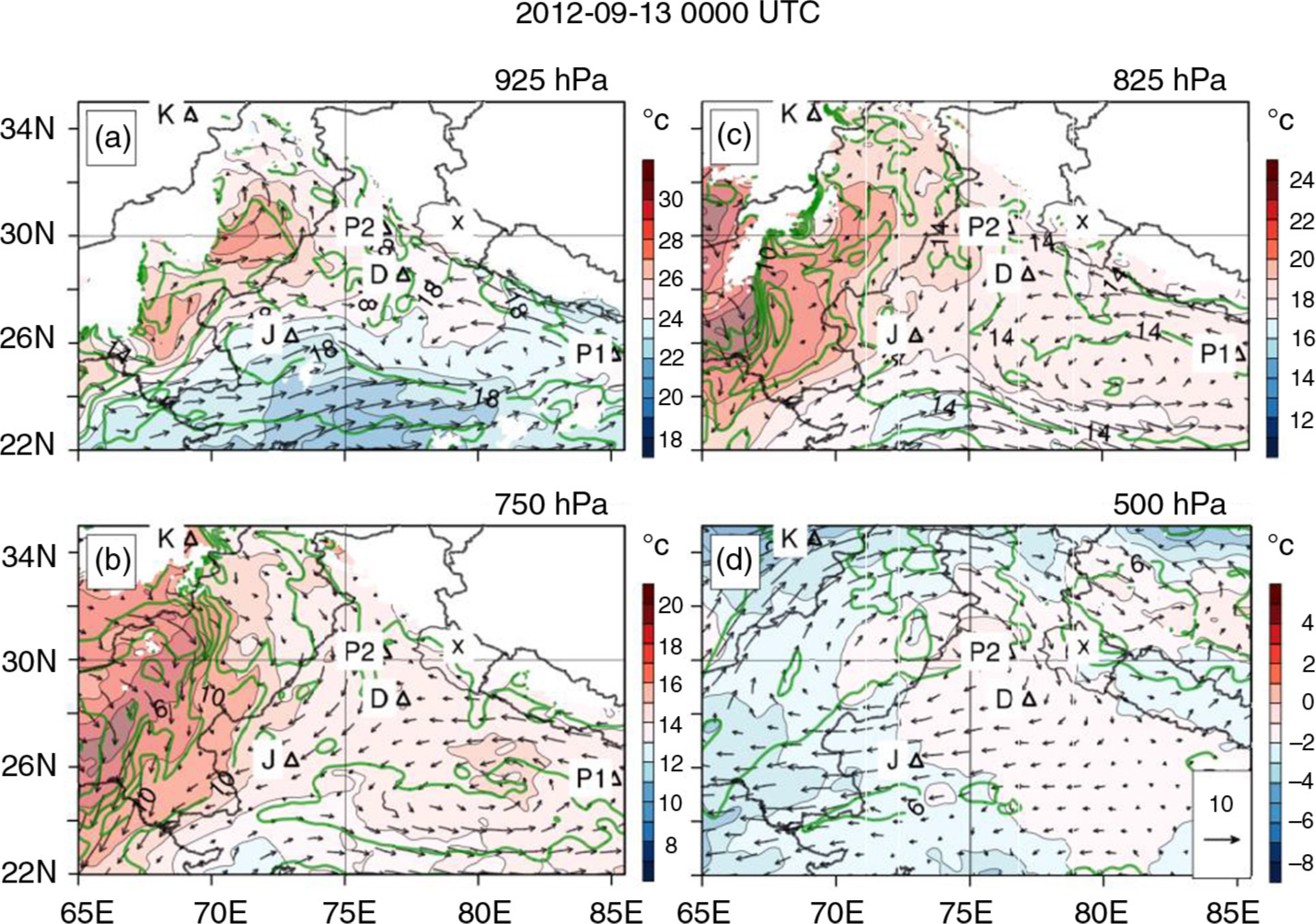
Fig. 4
Simulated atmospheric state variables for the D1 domain on 13 September 0:00 UTC: air temperature (K, colour shading), wind vectors (m/s, see scale in d) and water vapour mixing ratio (g/kg, green contour lines) at pressure levels a) 925 hPa, b) 750 hPa, c) 825 hPa and d) 500 hPa. The ‘x’ mark represents the Ukhimath town. The location of radiosonde stations over the domain in Jodhpur (J), Patna (P1), Delhi (D), Patiala (P2) and Kabul (K) are also marked.
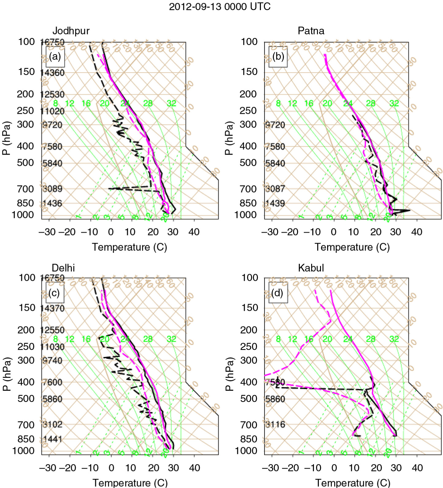
Fig. 5
Simulated (magenta) and measured (black) atmospheric soundings on 13 September 0000 UTC at (a) Jodhpur, (b) Patna, (c) Delhi and (d) Kabul. The model soundings were extracted from D1 domain for grid columns nearest to the sounding locations.
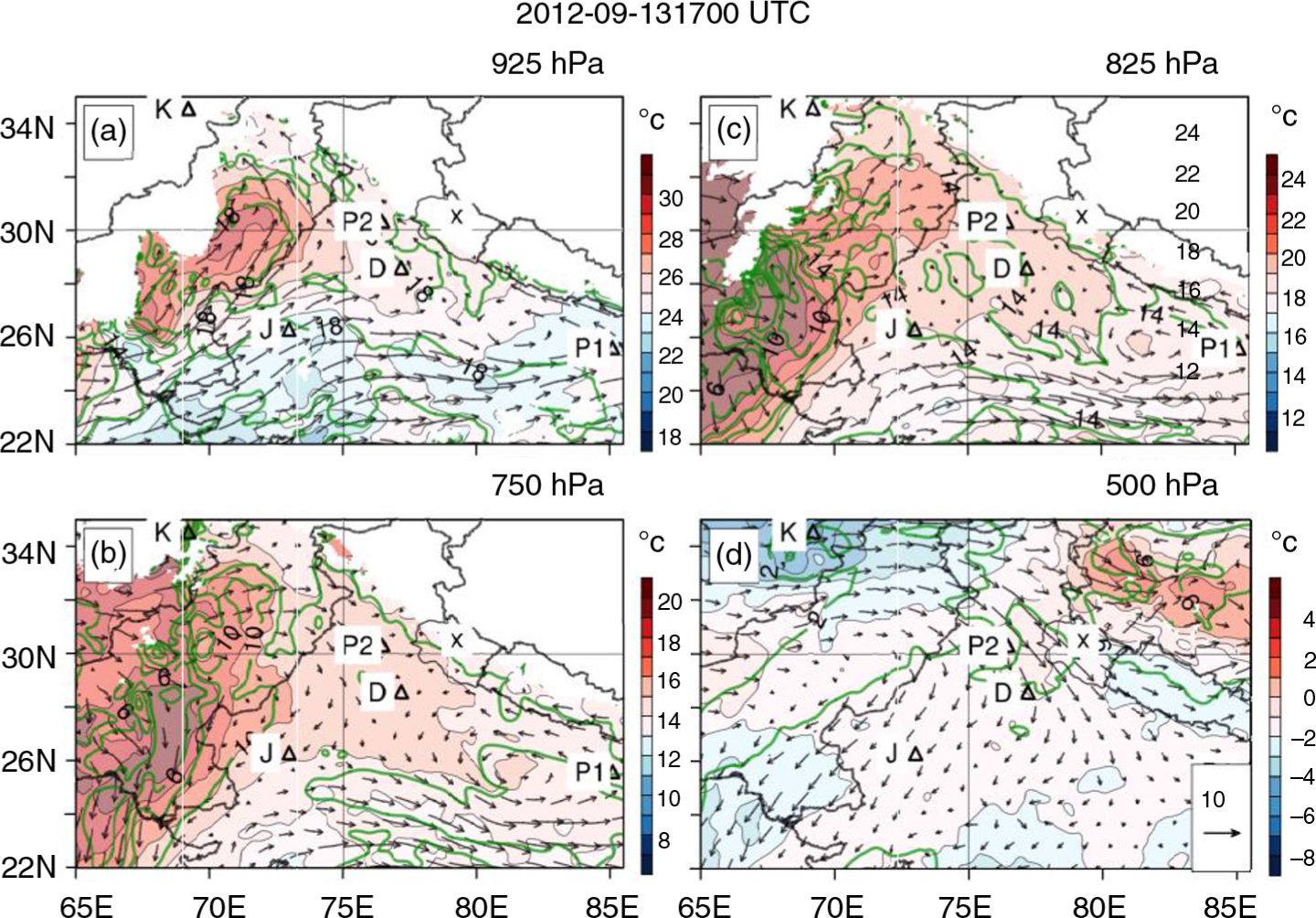
Fig. 6
Simulated atmospheric state variables for the D1 domain on 13 September 1700 UTC: air temperature (K, colour shading), wind vectors (m/s, see scale in d) and water vapour mixing ratio (g/kg, green contours) at pressure levels a) 925 hPa, b) 750 hPa, c) 825 hPa and d) 500 hPa. The ‘x’ mark represents the Ukhimath town. The location of radiosonde stations over the domain in Jodhpur (J), Patna (P1), Delhi (D), Patiala (P2) and Kabul (K) are also marked.
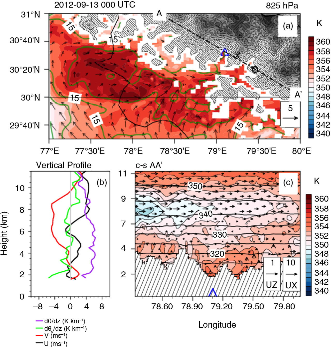
Fig. 7
(a) Simulated atmospheric state variables for the D2 domain on 13 September 0000 UTC: equivalent potential temperature (K, colour shading), wind vectors (m/s) and water vapour mixing ratio (g/kg, green contours) at 825 hPa. The ‘x’ and ‘o’ marks represents the Ukhimath town and the location of maximum precipitation, respectively. (b) Vertical profiles of averaged U and V wind components, gradients of potential temperature and equivalent potential temperature, along the cross-section AA’ in the valley upstream of Ukhimath town (indicated by Δ). (c) Cross-section AA’ of equivalent potential temperature (K, colour shading), wind vectors (m/s) and potential temperature (K, black contours).
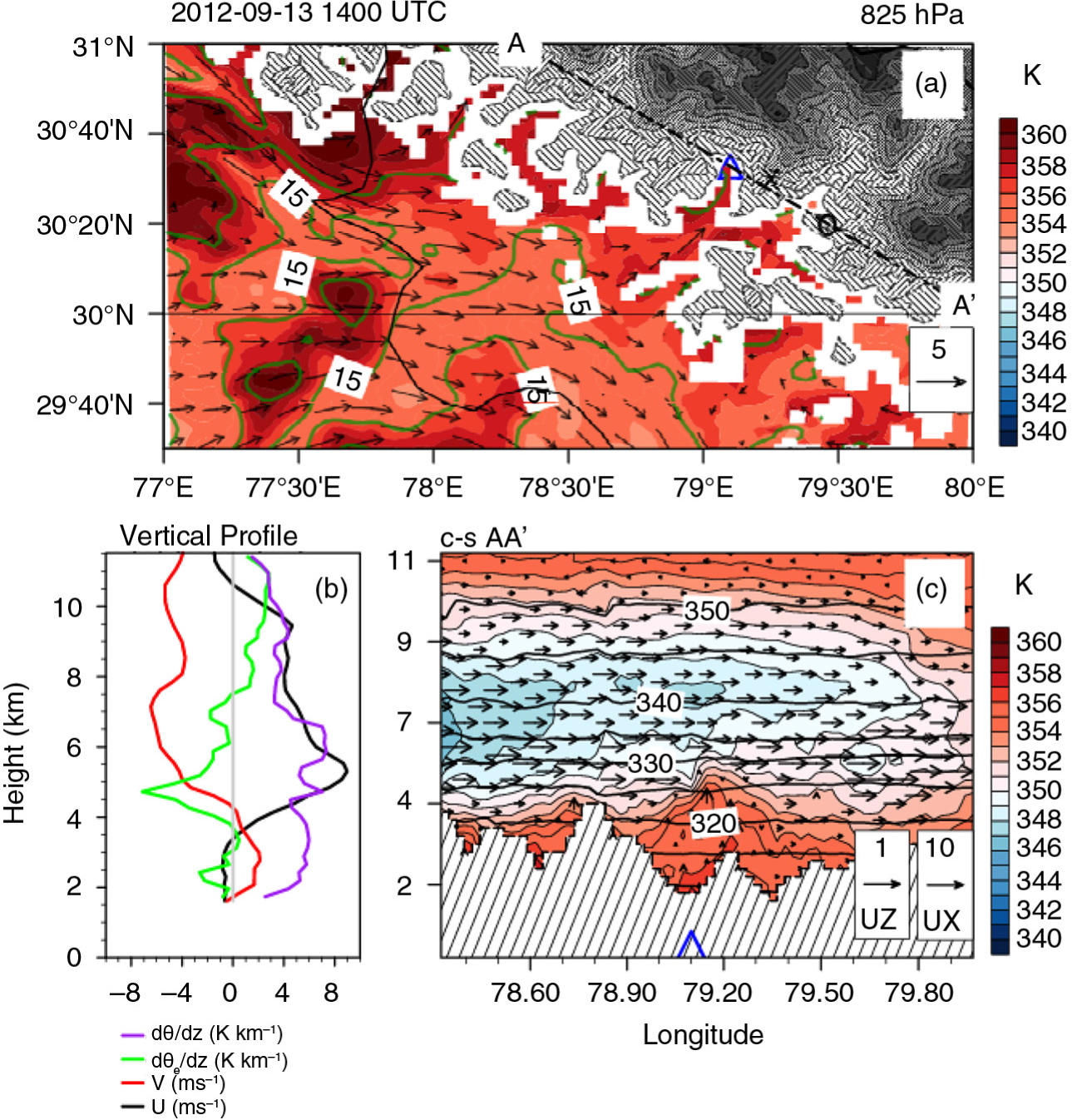
Fig. 8
(a) Simulated atmospheric state variables for the D2 domain on 13 September 1400 UTC: equivalent potential temperature (K, colour shading), wind vectors (m/s) and water vapour mixing ratio (g/kg, green contours) at 825 hPa. The ‘x’ and ‘o’ marks represent the Ukhimath town and the location of maximum precipitation, respectively. (b) Vertical profiles of averaged U and V winds, gradients of potential temperature and equivalent potential temperature, along the cross-section AA’ in the valley upstream of Ukhimath town (Δ). (c) Cross-section AA’ of equivalent potential temperature (K, colour shading), wind vectors (m/s) and potential temperature (K, black contours).
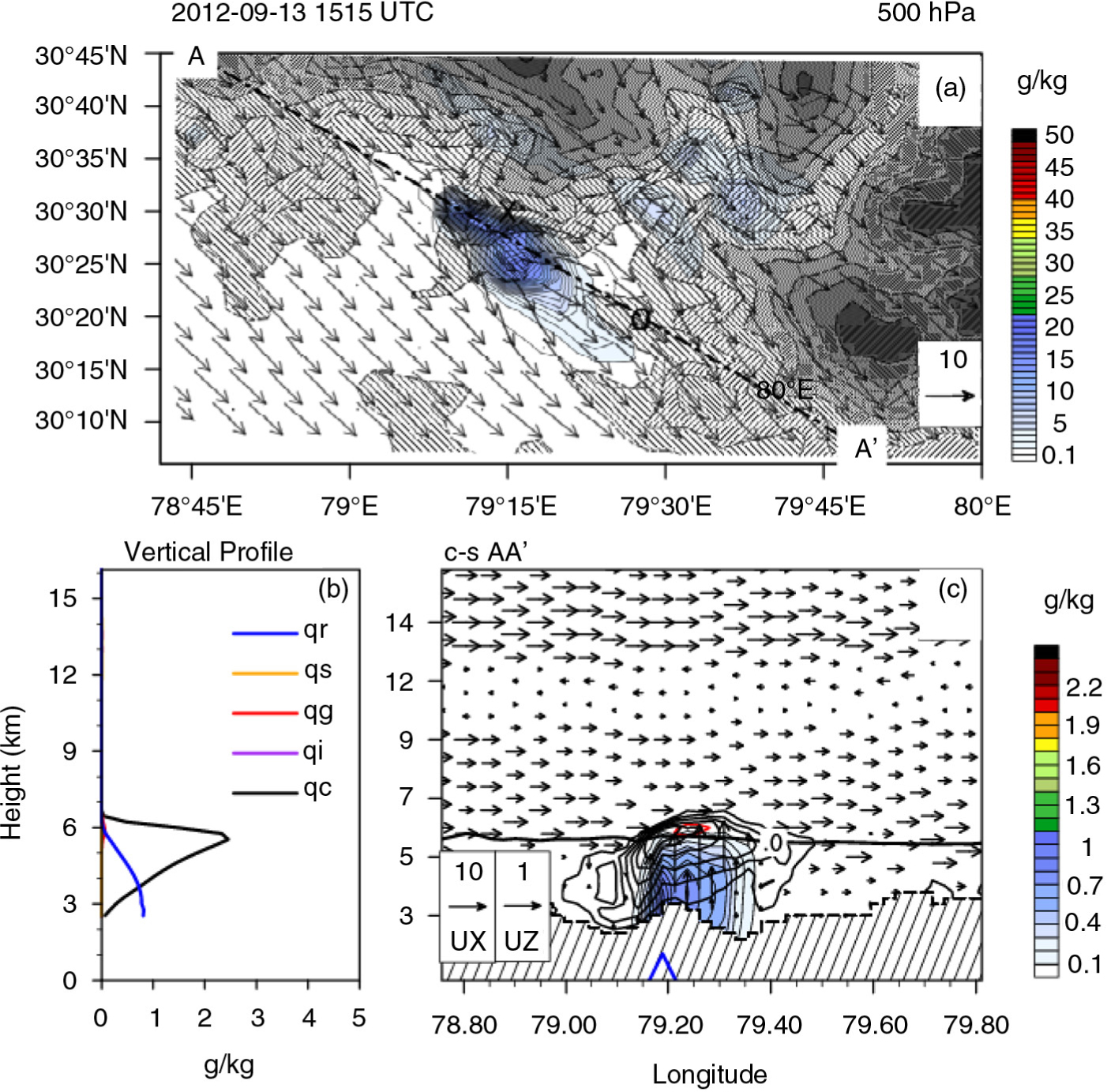
Fig. 9
(a) Simulated atmospheric state variables for the D2 domain on 13 September 1515 UTC: vertically integrated rain-water mixing ratio (g/kg, colour shading) and wind vectors (m/s) at 500 hPa. The ‘x’ and ‘o’ marks represent the Ukhimath town and the location of maximum precipitation, respectively. (b) Averaged vertical profiles of hydrometeors at precipitation maximum (Δ), along the cross-section AA’. (c) Cross-section AA’ of hydrometeors (qr in colour shading, qc, qi, qg, qs in solid lines from 0.2 to 2.4 g/kg at intervals of 0.4 g/kg), wind vectors and temperature (black contours, showing the melting level). [qx refers to mixing ratio of different hydrometeors, with x being cloud water (qc), cloud ice (qi), graupel (qg), snow (qs) and rain (qr)].
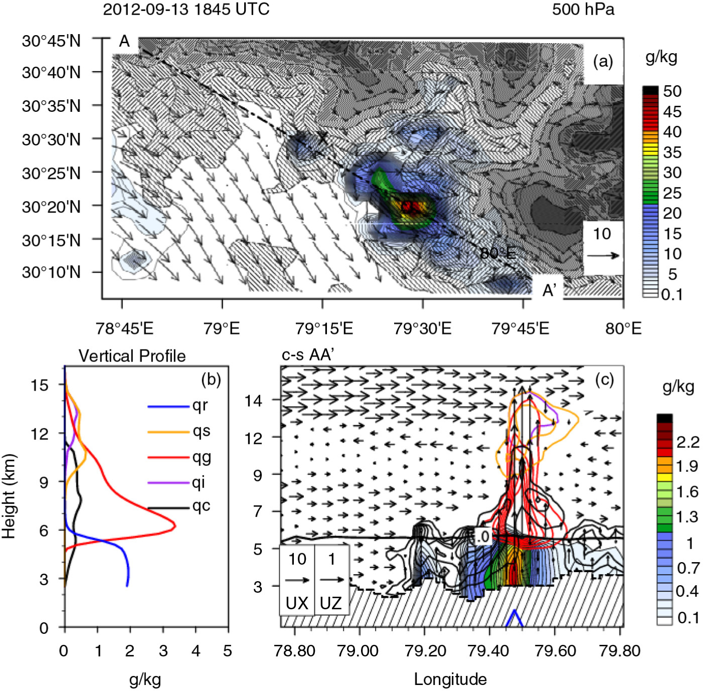
Fig. 10
(a) Simulated atmospheric state variables for the D2 domain on 13 September 1845 UTC: vertically integrated rainwater mixing ratio (g/kg, colour shading) and wind vectors (m/s) at 500 hPa. The ‘x’ and ‘o’ marks represent the Ukhimath town and the location of maximum precipitation, respectively. (b) Averaged vertical profile of hydrometeors at precipitation maximum (Δ), along the cross-section AA’. (c) Cross-section AA’ of hydrometeors (qr in colour shading, qc, qi, qg, qs in solid lines from 0.2 to 2.4 g/kg at intervals of 0.4 g/kg), wind vectors and temperature (black contours, showing the melting level). [qx refers to mixing ratio of different hydrometeors, with x being cloud water (qc), cloud ice (qi), graupel (qg), snow (qs) and rain (qr)].
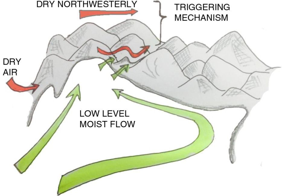
Fig. 11
Schematic of the meteorological setting and suggested mechanism for the occurrence of extreme rainfall event in Uttarakhand.