
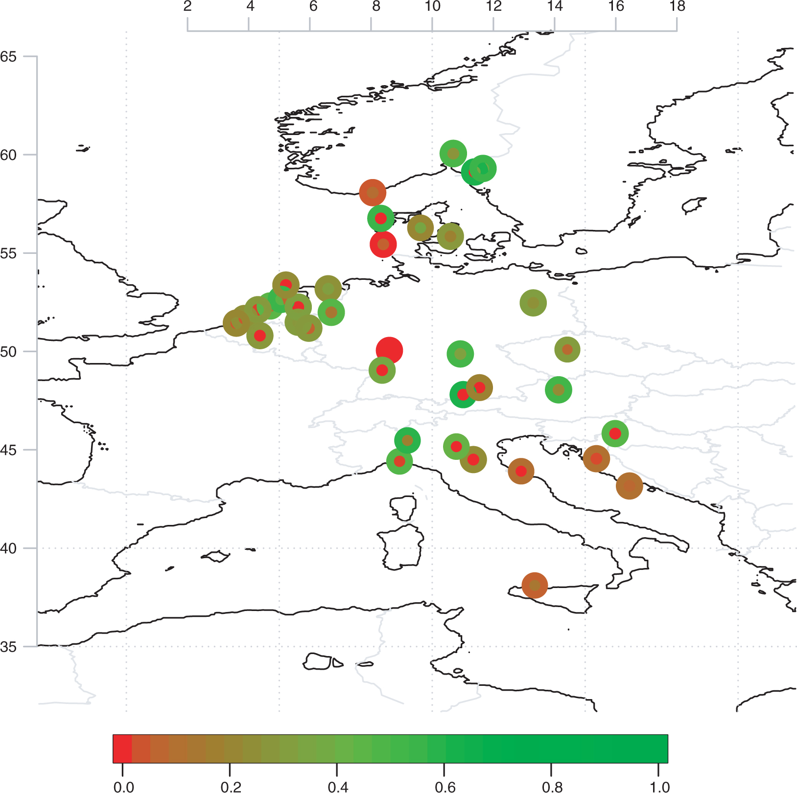
Fig. 1
The location of the rain gauge measurements for more than 130 yr. The size of the symbols is proportional to the number of valid data and their colour is according to the correlation between observed and predicted µ (inner part) or f w (outer part) over the independent period.
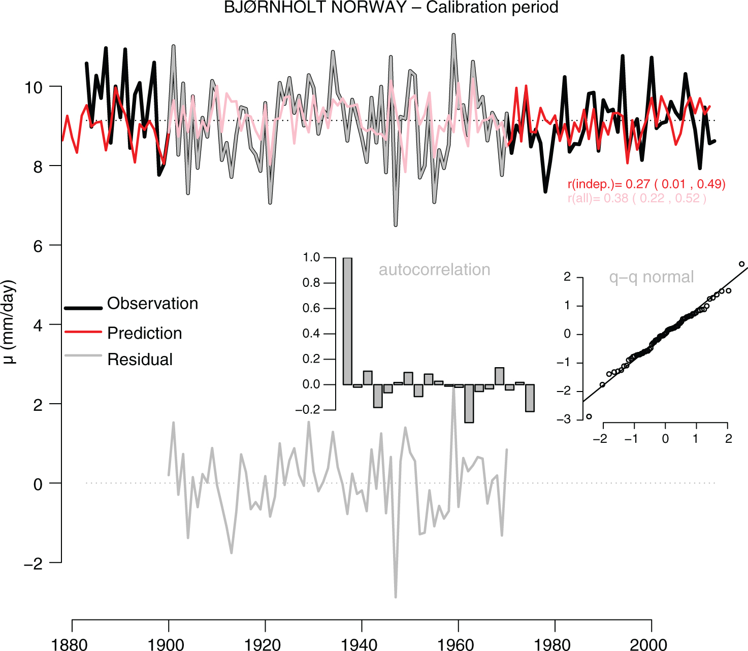
Fig. 2
An assessment of the downscaled µ. The upper part shows µ estimated from the rain gauge data (black) and predicted through the downscaling (red). The faint sections of the curves indicate the calibration interval. The correlation for the independent sections of the data are 0.27 the out-of-sample years and 0.38 for the entire curve, both statistically significant at the 5%-level. The lower part of the figure shows the residuals in grey, and the inserts show the auto-correlation function (ACF) and a q–q plot of the residuals against a normal distribution. The ACF indicates no persistence and the q–q plot suggest that the residuals follow the normal distribution closely.
Table 1. Summary of correlation scores: Annual (both for the independent out-of-sample and for all years), seasonal and pentads of wet-day mean (µ) of precipitation
BJØRNHOLT0.270.380.280.150.250.290.390.18BAMBERG0.330.410.300.110.160.230.130.57BERLIN-DAHLEM0.250.250.170.23−0.080.140.060.33BOLOGNA−0.020.070.110.110.04−0.04−0.13−0.29FRANKFURT−0.040.150.120.050.000.090.070.29GENOA0.010.240.270.240.07−0.070.13−0.05GOSPIC0.020.080.100.010.03−0.02−0.080.37GRONBAEK-ALLINGSKOVGARD0.350.210.180.010.130.100.010.26GRONINGEN-10.320.520.420.080.090.430.130.76HALDEN0.000.210.130.380.180.080.12−0.07HELMOND0.280.390.320.080.170.290.190.25HOHENPEISSENBERG−0.060.090.15−0.060.000.020.03−0.19HOOFDDORP0.130.120.090.130.080.270.090.06HOORN0.060.210.150.200.110.330.150.19HVAR0.070.090.010.110.050.06−0.07NAKARLSRUHE−0.040.100.11−0.070.140.060.080.14KERKWERVE0.320.350.330.160.020.320.180.62KREMSMUENSTER0.230.400.280.130.270.250.090.11MANTOVA−0.270.070.060.020.110.110.20NAMILAN0.180.360.300.040.040.180.27NAMUENCHEN−0.080.020.000.110.10−0.09−0.07−0.35NORDBY (FANO)0.060.04−0.060.180.13−0.040.160.03OKSOEY FYR0.090.260.240.260.010.15−0.100.34PALERMO0.140.410.320.240.15−0.050.21NAPESARO−0.120.060.04−0.090.07−0.050.13NAPRAHA-KLEMENTINUM0.080.170.04−0.23−0.110.070.09NAPUTTEN (GLD)−0.120.260.290.120.150.330.060.43ROERMOND0.060.280.290.010.160.220.120.35SCHEVENINGEN0.010.160.20−0.150.110.160.020.08STRØMSFOSS SLUSE0.420.360.270.040.040.190.180.37TRANEBJERG0.190.400.310.360.180.240.040.52UCCLE−0.200.110.030.290.030.100.12−0.12VESTERVIG−0.120.150.070.200.180.20−0.02−0.15VLISSINGEN-10.040.180.160.09−0.080.260.290.23WEST TERSCHELLING−0.090.370.260.330.150.250.000.30WINTERSWIJK0.140.380.300.130.11−0.020.160.35ZAGREB-GRIC−0.020.140.150.170.08−0.090.15−0.18
[i] The column ‘q 90’ provides the correlation scores for the predicted q 90 as in Fig. 8. The correlations for the seasons and pentads were for all years.
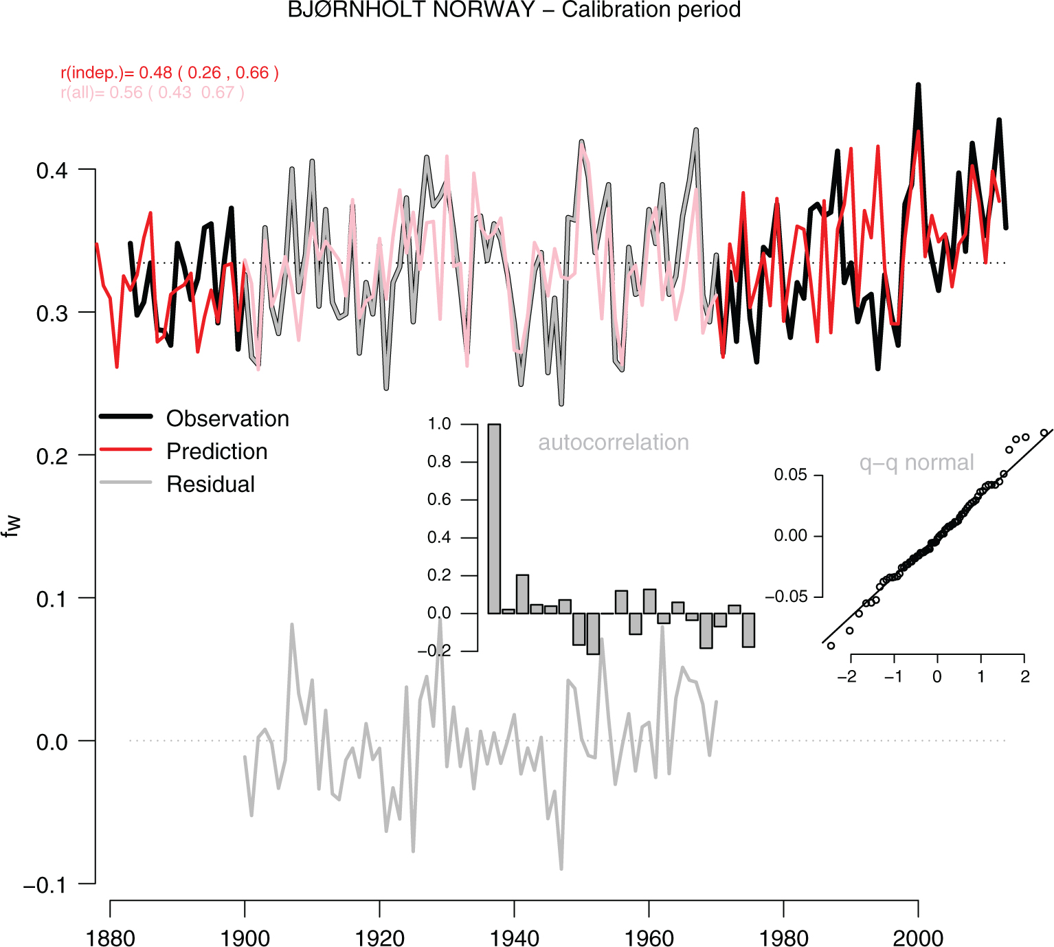
Fig. 3
Same as Fig. 2 but for f w . The correlation between the downscaled results and observed wet-day frequency is 0.48 (0.56 for the entire record) and statistically significant at the 5%-level. The two curves follow closely, albeit with periods of poorer match such as in the 1890s and 1990s. The residuals do not indicate the presence of persistence and appear to follow the normal distribution closely. Similar correlations for independent and the entire record suggest robust results.
Table 2. Summary of correlation scores. Annual, seasonal and pentads of wet-day frequency (f w ) of precipitation
BJØRNHOLT0.480.560.590.670.640.550.760.61BAMBERG0.510.570.460.490.480.230.660.41BERLIN-DAHLEM0.310.330.230.330.280.240.380.18BOLOGNA0.230.460.280.470.370.140.420.65FRANKFURT−0.100.180.160.130.100.070.510.19GENOA0.480.630.280.550.470.260.720.44GOSPIC0.110.400.410.300.380.280.360.32GRONBAEK-ALLINGSKOVGARD0.210.010.040.340.00−0.290.210.13GRONINGEN-10.260.440.300.690.660.400.66−0.05HALDEN0.630.600.440.400.580.370.720.09HELMOND0.300.470.400.670.550.370.66−0.03HOHENPEISSENBERG0.630.650.160.630.440.320.720.31HOOFDDORP0.450.570.230.620.740.480.700.21HOORN0.550.620.280.770.630.460.660.42HVAR0.110.500.440.500.310.240.340.67KARLSRUHE0.360.400.260.480.390.400.600.27KERKWERVE0.250.360.350.660.590.400.67−0.29KREMSMUENSTER0.520.630.330.640.580.360.600.39MANTOVA0.420.570.200.480.510.130.52NAMILAN0.590.710.440.520.540.350.62NAMUENCHEN0.190.300.100.470.290.310.460.22NORDBY (FANO)−0.06−0.070.10−0.41−0.14−0.16−0.06−0.03OKSOEY FYR0.040.330.200.160.470.380.290.33PALERMO0.060.200.210.350.230.260.24NAPESARO0.100.320.260.520.330.130.40NAPRAHA-KLEMENTINUM0.300.270.020.130.240.140.15NAPUTTEN (GLD)0.320.480.340.620.550.510.650.14ROERMOND0.290.410.280.550.520.300.66−0.08SCHEVENINGEN0.300.490.350.610.550.470.660.11STRØMSFOSS SLUSE0.410.520.440.540.570.460.680.16TRANEBJERG0.290.500.350.620.540.600.640.39UCCLE0.280.560.290.610.560.610.740.24VESTERVIG0.560.600.300.760.630.600.79−0.05VLISSINGEN-10.210.380.210.490.590.480.62−0.13WEST TERSCHELLING0.230.410.340.650.600.570.69−0.10WINTERSWIJK0.460.530.380.670.590.420.64−0.07ZAGREB-GRIC0.470.600.400.570.360.280.590.62
[i] The column ‘n(X>10mm)’ shows the correlation between the median number of days with rainfall greater than 10 mm/day as in Fig. 9. There was a bias for some stations that gave a shift in the predicted 90% confidence interval even with moderately high correlations. The correlations for the seasons and pentads were for all years.
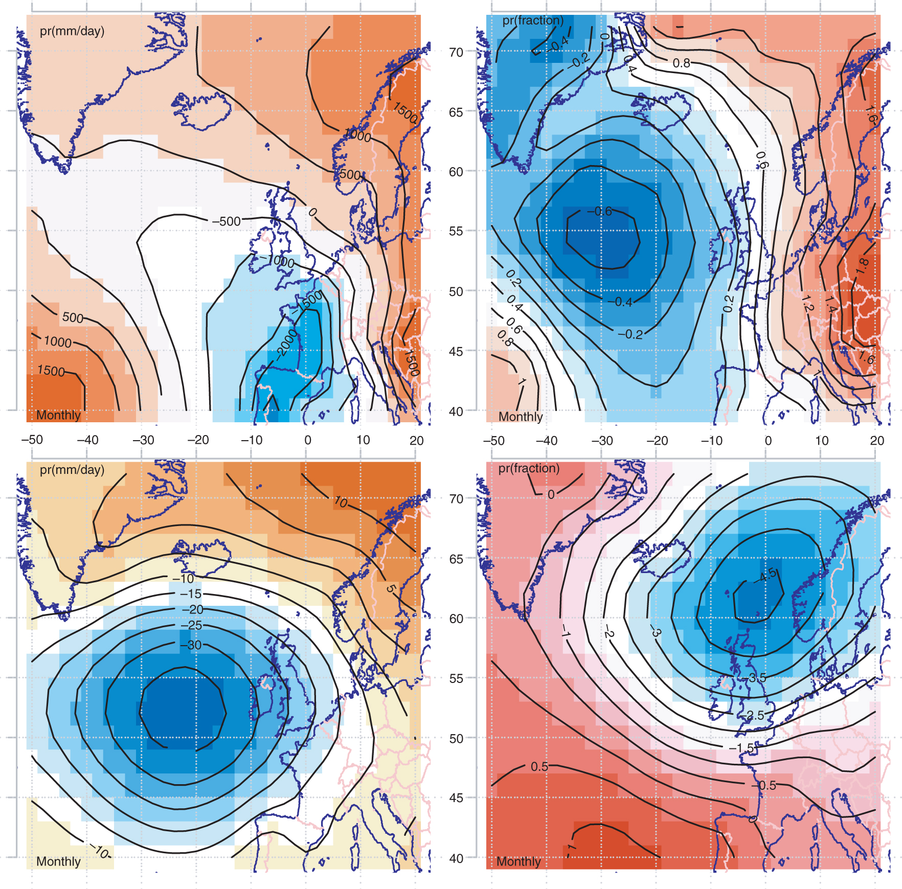
Fig. 4
Maps showing the spatial SAT (upper) and SLP (lower) anomalies associated with variations in µ (left) and f w (right).
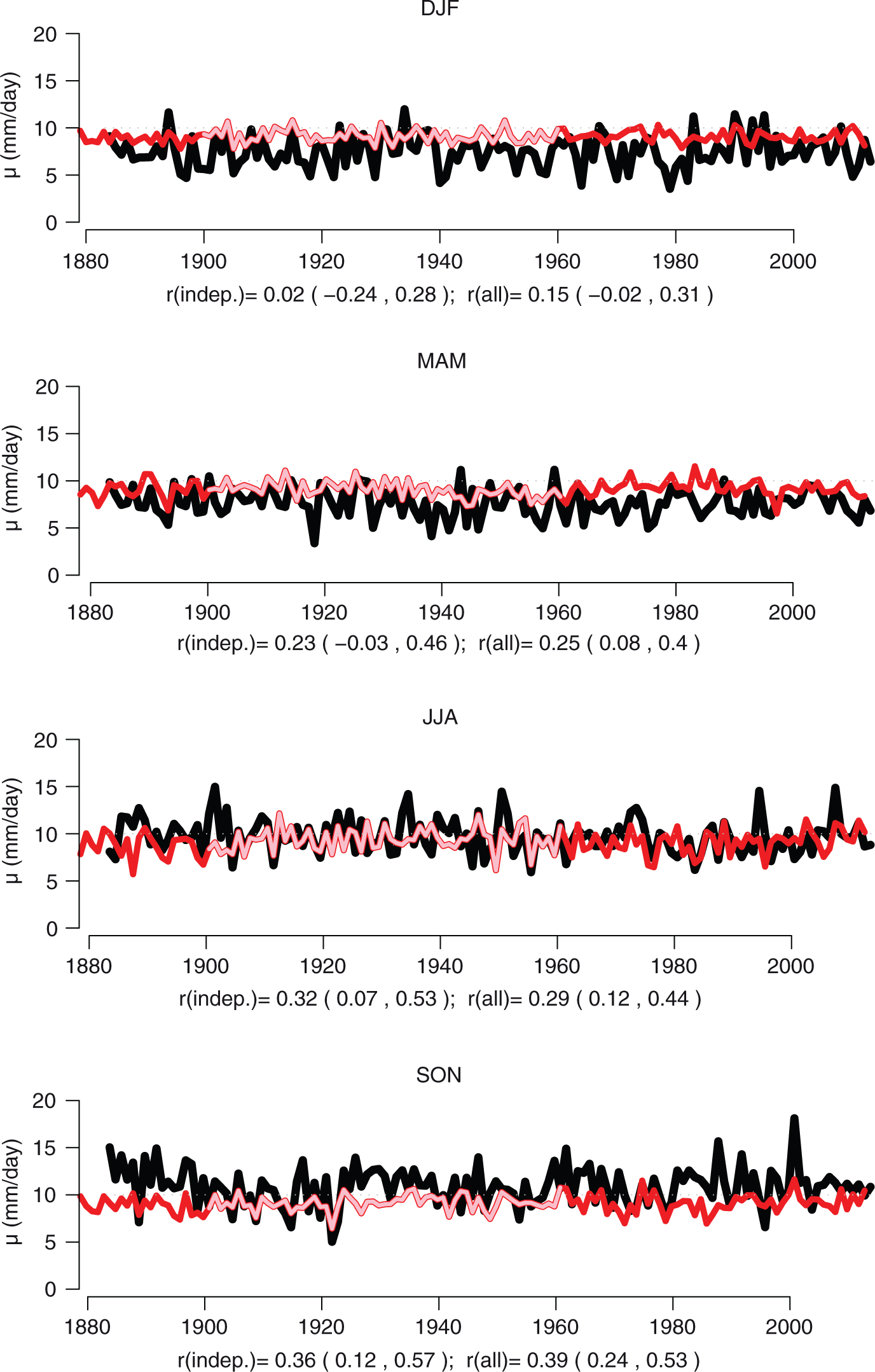
Fig. 5
A comparison between seasonal µ for the four seasons and corresponding values predicted through the downscaling (red). The section of curves with faint colours indicate the calibration period. The correlation is distinguishable from zero only in summer. The results do not indicate that a model calibrated on annual data is valid for sub-annual time scales. Similar correlations for independent and the entire record suggest robust results.
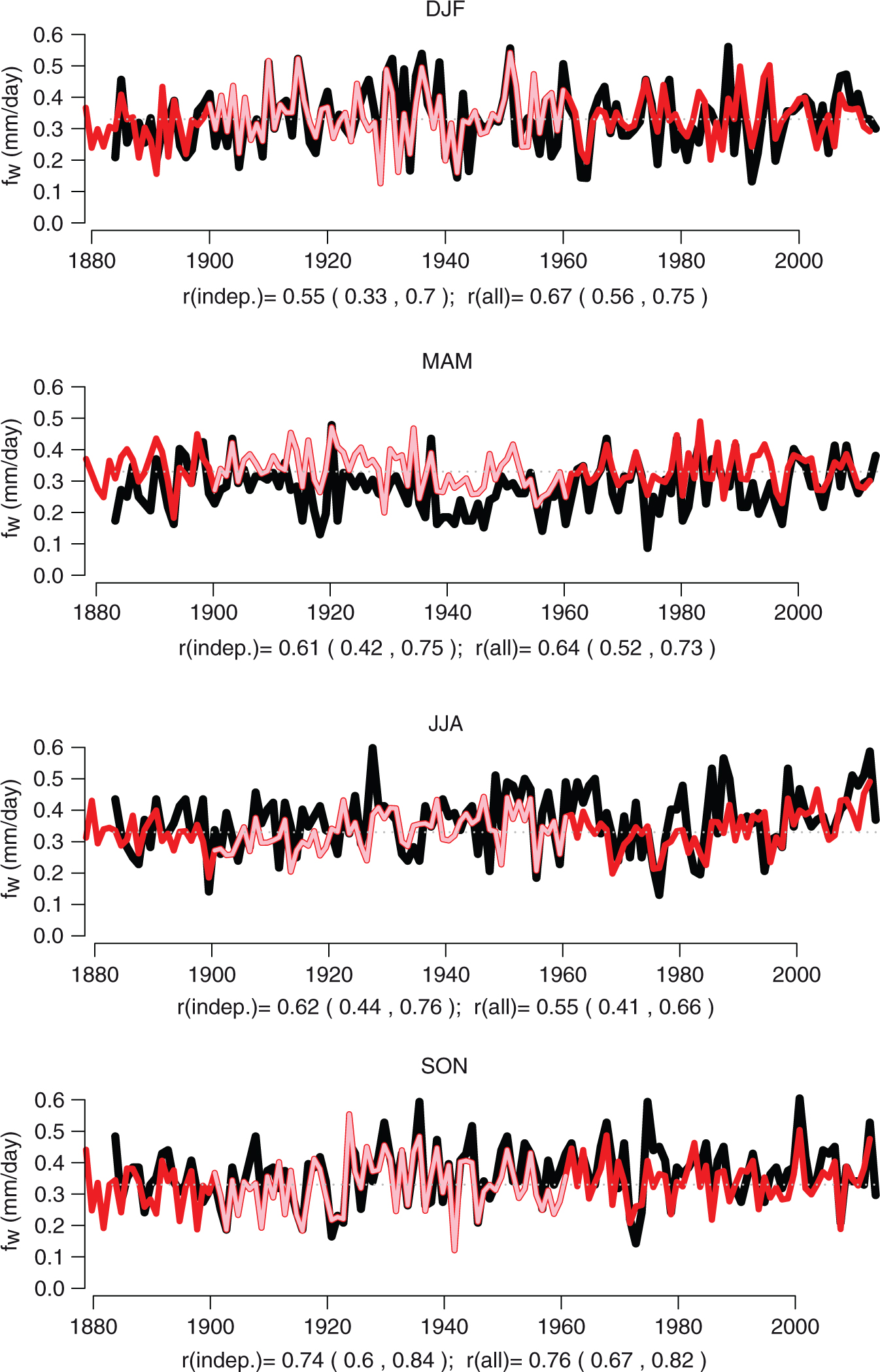
Fig. 6
A comparison between seasonal f w for the four seasons and corresponding values predicted through the downscaling (red). The section of curves with faint colours indicate the calibration period. The correlation is distinguishable from zero only in summer. The results indicate that a model calibrated on annual data is valid for sub-annual time scales. Similar correlations for independent and the entire record suggest robust results.

Fig. 7
Same as Fig. 2 but for pentads. The residual does not suggest any persistence and is close to being normally distributed, after a third regression against the global mean temperature was included. There is a modest correlation between the predictions and observations, but the results do not indicate that a model calibrated on annual data is valid for multi-annual time scales.

Fig. 8
A comparison between observed wet-day 95-percentile q 95 and corresponding values estimated from µ (grey) and through downscaling (red) using SAT and SLP as predictors. The method appears to capture some of the multiyear variations but not some of the most pronounced the individual spikes.
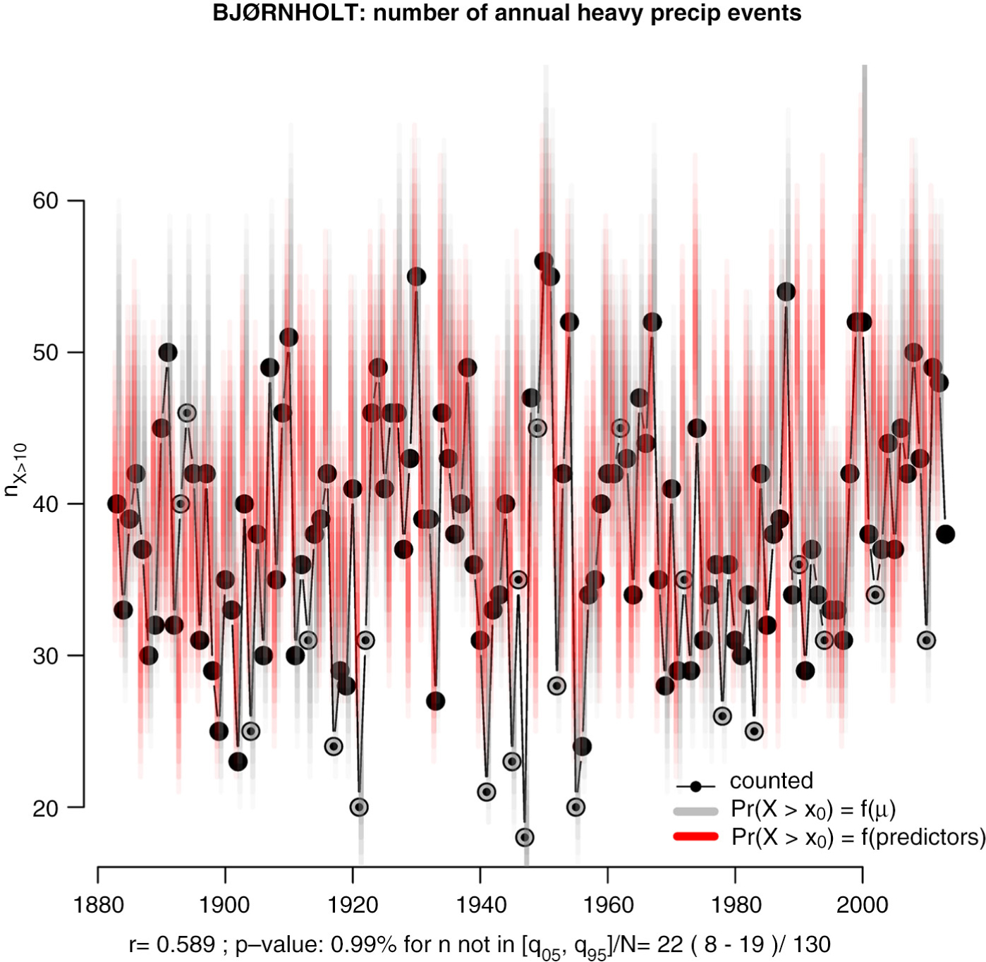
Fig. 9
Predicted and observed number of intense precipitation events, defined by exceeding the threshold value x 0=10mm/day. Symbols represent the counted events based on rain gauge data, grey shading the 90% confidence interval implied by µ and f w derived from the observations, and red shading the 90% confidence interval derived through the downscaling exercise. The confidence intervals were derived taking the 5 and 95% percentiles from a binomial distribution where the probability for exceeding the 10 mm/day was taken from eq. (A4). The filled symbols mark the years when the number of events was outside the 90% confidence interval.

Fig. 10
A measure of skill. The right axis and the thick line indicate the number of observed events that were outside the predicted 90% confidence interval for a range of different threshold values x 0 (x-axis). The left axis and thin lines indicate the probability associated with the observed number of intense wet events outside the predicted 5–95% annual interval estimated according to a binomial distribution. The number of years with events outside the confidence interval are counted and then the probability is estimated according to the binomial distribution, the sample size (number of years), and a probability of 10% for being outside the predicted 90% confidence interval. The red curves show results from the downscaling exercise whereas the grey curves show the results derived from µ and f w estimated directly from the rain gauge data.
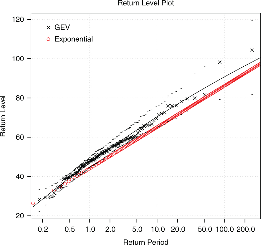
Fig. A1
A comparison between return values derived from GEV and eq. (A6) for Bjørnholt suggests that the exponential distribution has a tendency to under-estimate the return-levels. Still, the ‘error’ associated with the estimates based on the simpler expression for are less than 10% compared with the GEV-based estimates (not shown). Hence, a rough estimate for return-levels can be obtained by downscaling the wet-day mean µ and frequency f w .