
Fig. 1
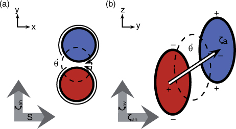
Schematic overview of PV dipoles generated due to convection, diabatic perturbation indicated by dashed black circle and positive (negative) PV pole indicated by red (blue) circle. The±signs indicate regions of high and low static stability, and the direction of the (dominant) horizontal vorticity vector. (a) Horizontal cross section, PV dipoles created in the direction of absolute vorticity k×S, with S the vertical wind shear. Storm-relative wind velocities associated with the PV anomalies are indicated by black arrows. (b) Vertical cross section along the direction of k×S.
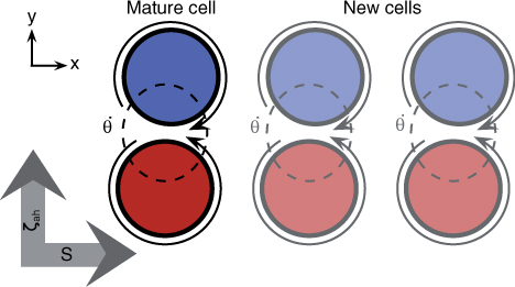
Fig. 2
As in Fig. 1, a diabatic perturbation is indicated by a dashed black circle and a positive (negative) PV pole by a red (blue) circle. New cells (transparent) are preferentially generated downshear, which could, in combination with advection, lead to bands of positive and negative PV.
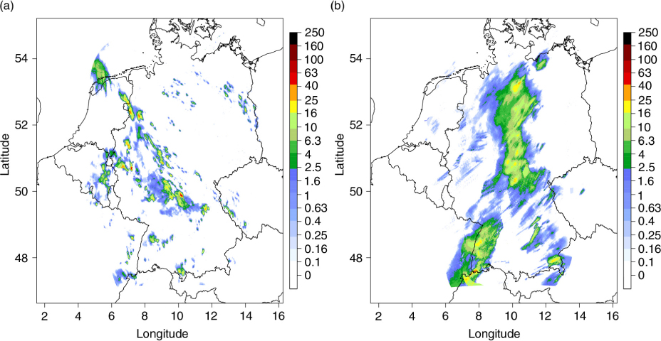
Fig. 3
Rain rates in millimetre per hour, using RADOLAN RW data (Bartels et al., 2004) for (a) 5 June and (b) 22 June 2011 at 14:50 UTC, respectively.
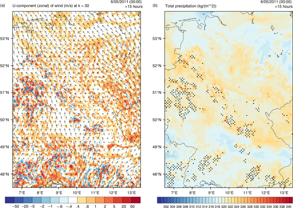
Fig. 4
(a) PV (contours) and wind flow (arrows). (b) Equivalent potential temperature and precipitation (dots indicate hourly precipitation rates above 0.5 mm, dashed patterns above 5.0 mm in the previous hour). Both plots on 5 June 2011 at 15 UTC at model level 30 (about 3 km).
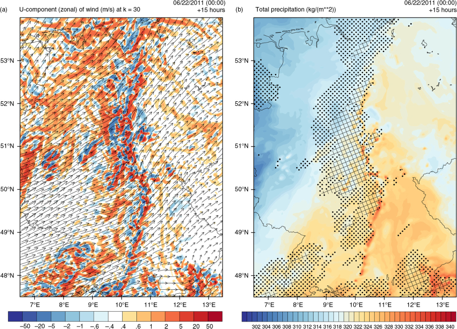
Fig. 5
(a) PV (contours) and wind flow (arrows). (b) Equivalent potential temperature and precipitation (dots indicate precipitation above 0.5 mm, dashed patterns above 5.0 mm in the previous hour). Both plots on 22 June 2011 at 15 UTC at model level 30 (about 3 km).
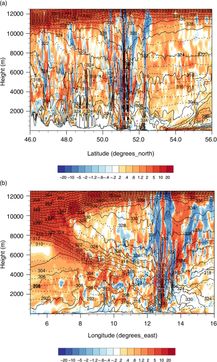
Fig. 6
Figures (a) and (b) show the PV (contours), the equivalent potential temperature θ e (dashed contour lines) and potential temperature θ (solid contour lines) for a longitudinal cross section at 7° at 5 June 2011 at 15 UTC and a latitudinal cross section at 52° for 22 June 2011 at 18 UTC.
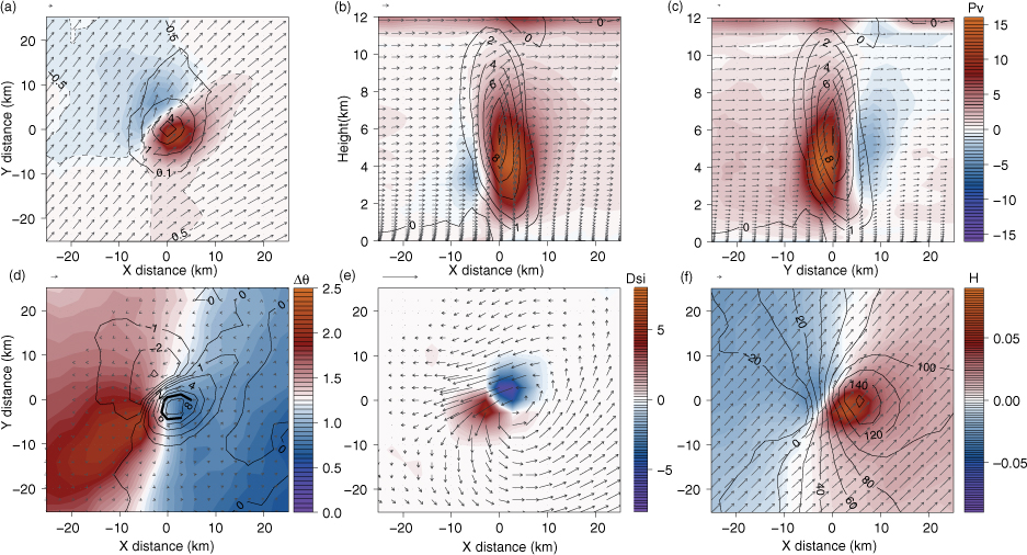
Fig. 7
(a) 3–7.3 km height integrated composites of PV (contours, in PVU), vertical velocity (contour lines, in ms−1) and 0–6 km wind difference (arrows) for 22 June 2011 at 15 UTC. Dashed lines indicate PV contours of −0.5 PVU and 0.5 PVU. (b) Longitudinal cross section at 0 km of (a), with PV (contours, in PVU), vertical wind (black contours, in ms−1) and wind velocity (arrows) for 22 June 2011 at 15 UTC. (c) as (b), but latitudinal cross sections at 0 km. (d) θ difference in the lowest 500 m (contours, in δ K), 3–7.3 km height integrated PV (black contours, in PVU) and wind velocity (arrows) for 22 June 2011 at 15 UTC. (e) 3–7.3 km height integrated composites of DSI (contours, in PVU2s−1) and perturbation wind (arrows) for 22 June 2011 at 15 UTC. (f) 3–7.3 km height integrated composites of helicity H (contours, in ms−2), 0–3 km SRH (black contour lines) and full wind velocity (arrows) for 22 June 2011 at 15 UTC. Reference arrow at top of each plot of 5 ms−1.
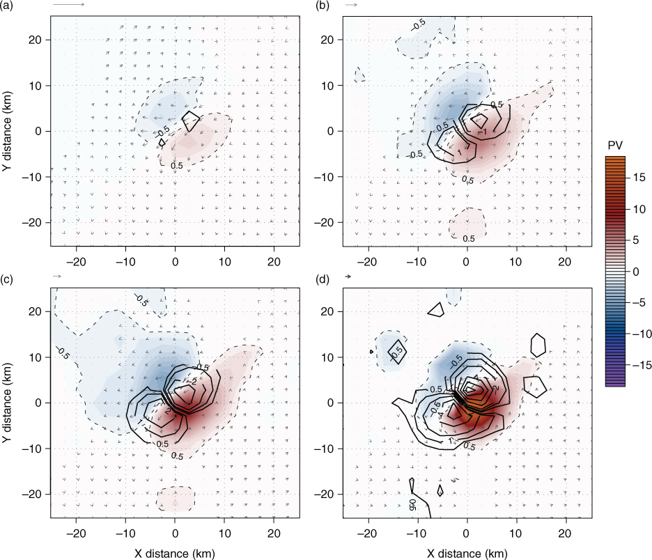
Fig. 8
3–7.3 km height integrated composites for 22 June 2011 at 15 UTC of PV (contours, in PVU), DSI (black contour lines, in PVU2s−1) and perturbation wind for height averaged vertical velocity threshold of (a) 1–3 ms−1, (b) 3–5 ms−1, (c) 5–10 ms−1 and (d) above 10 ms−1.
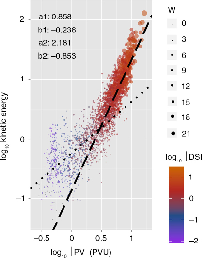
Fig. 9
3–7.3 km height averaged against height averaged (in a 7×7 grid point domain around updraft) for 22 June 2011 at 15 UTC. Height averaged and vertical velocity (ms−1) indicated by dot colour and dot size, respectively. Fit of indicated in plot, for cells with (a1, b1, dotted line) and cells for which (a2, b2, dashed line).
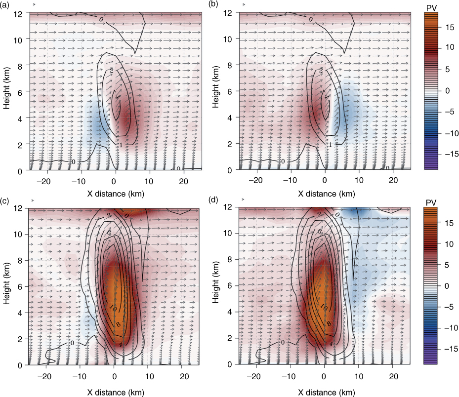
Fig. 10
(a) Longitudinal cross section for composites using a height average vertical velocity threshold of 3–5 ms−1 for 22 June 2011 at 15 UTC (at 0 km of Fig. 8b). PV indicated by contours (in PVU), vertical wind by black contours (in ms−1) and wind velocity by arrows. (b) as (a), but latitudinal cross sections at 0 km. (c–d) as (a–b) but for composites with a vertical velocity threshold above 10 ms−1.
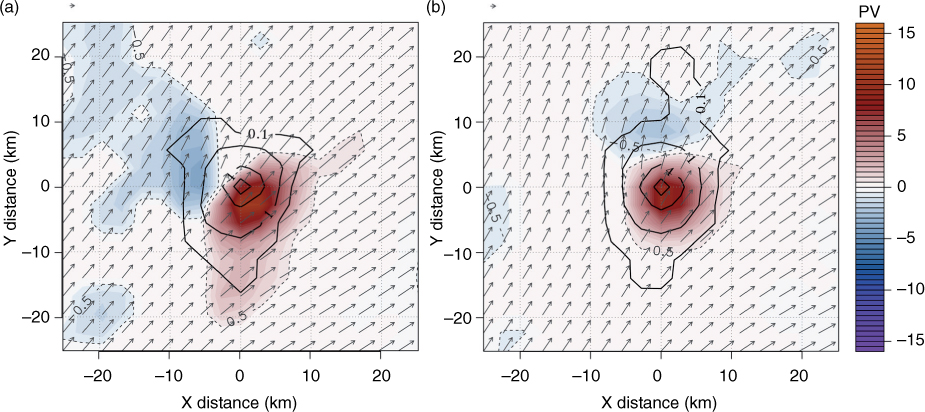
Fig. 11
(a) 3–7.3 km height integrated composites of PV (contours, in PVU), vertical velocity (contour lines, in ms−1) and 0–6 km wind difference (arrows) for 22 June 2011 at 11 UTC. (b) Same as (a) but for 22 June 2011 at 18 UTC. Reference arrow at top of each plot indicates a wind speed of 5 ms−1.
Table 1. Storm cell characteristics at 22 June 2011, calculated over all storm updrafts for all ensemble members
111323.77/15.53/34.50−28.11/ − 13.11/ − 3.430.43122535.98/16.48/30.64−26.93/ − 13.20/ − 4.110.36133996.53/16.43/29.58−23.30/ − 13.12/ − 4.490.45145497.48/16.63/32.34−24.48/ − 13.76/ − 5.200.45155966.95/17.48/35.37−22.87/ − 13.08/ − 5.420.49166136.68/17.10/32.84−25.38/ − 12.82/ − 4.580.50175526.08/16.82/35.04−22.54/ − 11.97/ − 4.040.52184545.66/15.61/31.21−22.23/ − 10.95/ − 4.280.57193905.68/15.78/30.57−21.83/ − 11.22/ − 4.250.54
[i] Maximum and minimum PV (in PVU) are searched in a 3×3 gridpoint surroundings of the vertical velocity maximum. The correlation coefficient between W and PV is calculated with eq. (4), following Davies-Jones (1984).
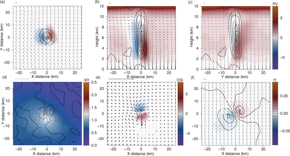
Fig. 12
(a) 3–7.3 km height integrated composites of PV (contours, in PVU), vertical velocity (contour lines, in ms−1) and 0–6 km wind difference (arrows) for 5 June 2011 at 15 UTC. Dashed lines indicate PV contours of −0.5 PVU and 0.5 PVU. (b) Longitudinal cross section at 0 km of (a), with PV (contours, in PVU), vertical wind (black contours, in ms−1) and wind velocity (arrows) for 5 June 2011 at 15 UTC. (c) as (b), but latitudinal cross sections at 0 km. (d) θ difference in the lowest 500 m (contours, in δ K), 3–7.3 km height integrated PV (black contours, in PVU) and wind velocity (arrows) for 5 June 2011 at 15 UTC. (e) 3–7.3 km height integrated composites of DSI (contours, in PVU2s−1) and perturbation wind (arrows) for 5 June 2011 at 15 UTC. (f) 3–7.3 km height integrated composites of helicity H (contours, in ms−2), 0–3 km SRH (black contour lines) and full wind velocity (arrows) for 5 June 2011 at 15 UTC. Reference arrow at top of each plot of 5 ms−1.
Table 2. Storm cell characteristics at 5 June 2011, calculated over all storm updrafts for all ensemble members. Maximum and minimum PV (in PVU) are searched in a 3×3 gridpoint surroundings of the vertical velocity maximum. The correlation coefficient between W and PV is calculated with Eq. 4, following Davies-Jones (1984)
113891.53/5.69/12.33−12.58/ − 5.72/ − 1.530.02128071.36/5.59/12.25−12.53/ − 5.91/ − 1.520.041312251.74/6.75/14.16−14.69/ − 6.97/ − 1.810.061414791.94/7.29/15.72−14.64/ − 7.23/ − 2.000.071514211.97/7.87/17.29−16.00/ − 7.76/ − 2.110.081612451.85/8.40/19.02−17.00/ − 7.81/ − 1.920.12179661.74/8.31/18.31−16.37/ − 7.61/ − 1.880.13186531.80/8.24/18.56−16.35/ − 7.65/ − 1.950.12195282.01/8.11/18.20−16.62/ − 7.25/ − 2.090.13