
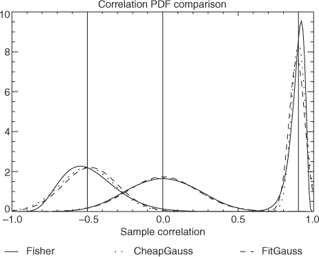
Fig. 1
Different approximations to the distribution of sample correlations for 20 ensemble members given true correlations of 0.0, −0.5 and +0.9 (indicated by vertical lines). The curves show the PDF implied by the Fisher transform (solid), a Gaussian with mean and standard deviation given by the cheap approximation introduced in Section 2.2 (dotted), and a Gaussian whose parameters are obtained by numerical integration of the Fisher transform (dashed).
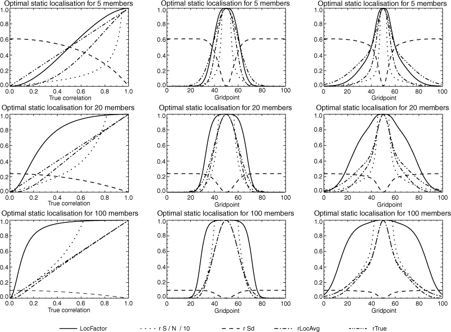
Fig. 2
The steps of the simplified optimal localisation calculation for 5 (top), 20 (middle) and 100 (bottom) ensemble members, showing the universal function of the true correlation (left), and results as a function of gridpoint where the true correlation varies as a Gaussian with half-width 10 gridpoints (middle) or an average of Gaussians with half-widths of 5 and 20 gridpoints (right). The lines show the true correlation (double-dot–dashed), approximated standard deviation of sample correlations (dashed), signal-to-noise ratio Q (dotted, divided by 10 for convenience of plotting), calculated optimal localisation factor (solid) and mean localised correlation (dot–dashed).

Fig. 3
RMS analysis error as a function of the half-width (in gridpoints) of a Gaussian-shaped localisation function, and also for the simplified optimal localisation (‘STheory’), and, in one case, optimal localisation with numerical evaluation of the full Fisher integrals (‘CTheory’). In (a) the true correlation is a Gaussian with a half-width of five gridpoints; in (b) it is the average of Gaussians with half-widths of 5 and 20 gridpoints, with observation error variance halved; in (c) the half-width varies linearly from 5 to 20 gridpoints across the domain; (d) is like (a) except the observation standard deviation is trebled and variance sampling errors are artificially removed to match the assumptions of the optimal localisation calculation. Results are shown for observation spacings of 40 (solid), 20 (dotted), 5 (dashed) and 2 [dot–dashed, omitted for case (c)] gridpoints. All tests use five ensemble members.
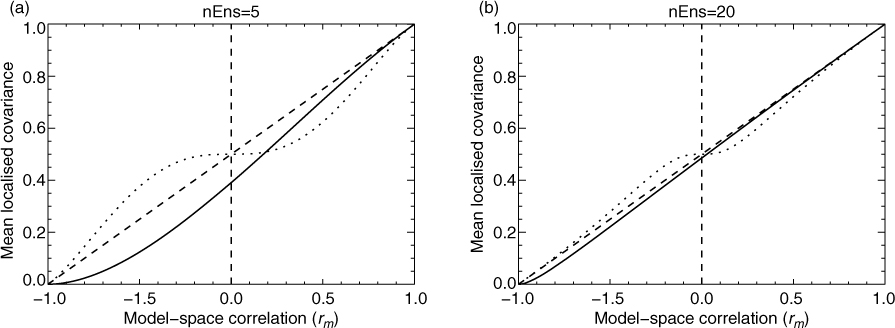
Fig. 4
Mean localised covariances between modelled and observed quantities for two gridpoints with model-space correlation r m , H=(0.5, 0.5), and ensembles with (a) 5 and (b) 20 members, resulting from optimal observation-space localisation (, solid) and the model-space localisation (, dotted) that is optimal for point observations. The dashed diagonal lines show the true covariance, P f H T , and the simplified optimal localisation calculation is used throughout.
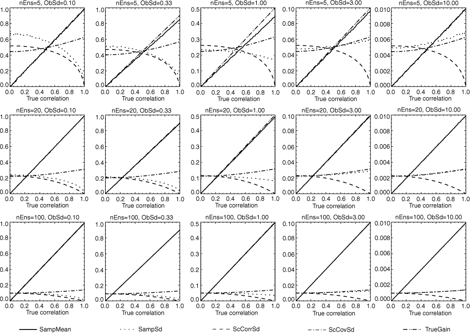
Fig. 5
The mean (solid) and standard deviation (dotted) of the sample gain calculated from ensembles of 5 (top), 20 (middle) or 100 (bottom) members, as a function of the true correlation (r) between the two points, with unit background error variances and observation standard deviations of 0.1, 0.33, 1.0, 3.0 and 10.0 (left to right). Additional lines indicate the gain implied by the true covariances (double-dot–dashed), and the standard deviation expected when the sampling error is associated with the correlation alone [dashed, by numerical integration with derived from eq. (9)], or the covariance alone [dot–dashed, using eq. (15)].
Table 1. The empirically determined optimal covariance localisation factor(s) between two gridpoints with background error correlation r and unit variances, where either one (nObs=1) or both (nObs=2) points are directly observed
nObsFactor0.200.500.75
1α0.450.901.002α0.450.850.952αu 0.250.700.90αd 0.050.450.75
[i] For nObs=2, the system can be forced to use a single localisation factor (α), or allowed to choose separate values for the numerator (α u ) and denominator (α d ) of eq. (11). The listed values achieved the lowest RMS error from the set 0, 0.05, …, 1 with 105 runs each, 20 ensemble members, and variance errors artificially removed.
Table 2. The empirically determined optimal covariance localisation factors between three gridpoints, two of which are observed, with background error correlation r 1 between the observed points, r 2 between the observed and unobserved points, and unit variances
Factorr20.200.500.75
αu1 0.200.20.60.90.500.40.60.90.750.60.70.9αu2 0.200.40.40.40.500.90.80.80.751.00.90.9αd1 0.200.00.30.70.500.40.30.70.750.80.50.7
[i] The system is allowed to choose separate localisation factors for r 1 (α u1 ) and r 2 (α u2 ) in the numerator and r 1 in the denominator (α d1 ) of eq. (11). The listed values achieved the lowest RMS error from the set 0, 0.1, …, 1 with 105 runs each, 20 ensemble members, and variance errors artificially removed.