
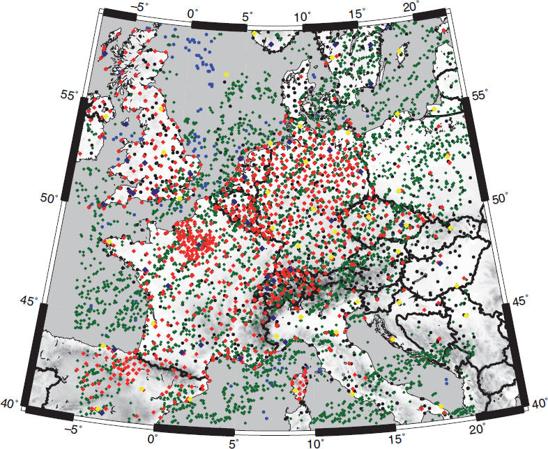
Fig. 1
Model domain, observation types, and their locations for the assimilation at 00 UTC, 26 September 2012. Black=Surface stations (SYNOP+Metar), blue=ship observations (SHIP), green=aircraft observations and atmospheric motion vectors from satellite (AMDAR+SATOB), red=GPS zenith total delay, yellow=radiosondes (TEMP) and brown=wind profiler.
Table 1. Parameterisation schemes applied for the WRF QPE experiment
Long wave radiationRRTMG (Iacono et al., 2008) Short wave radiationRRTMG (Iacono et al., 2008) Deep convectionSimulated explicitlyShallow convectionGRIMS (Hong et al., 2013) Cloud microphysicsMorrison 2-moment (Morrison et al., 2009) Planetary boundary layer (turbulence)YSU (Hong et al., 2006) Land surface schemeNoah-MP (Niu et al., 2011)
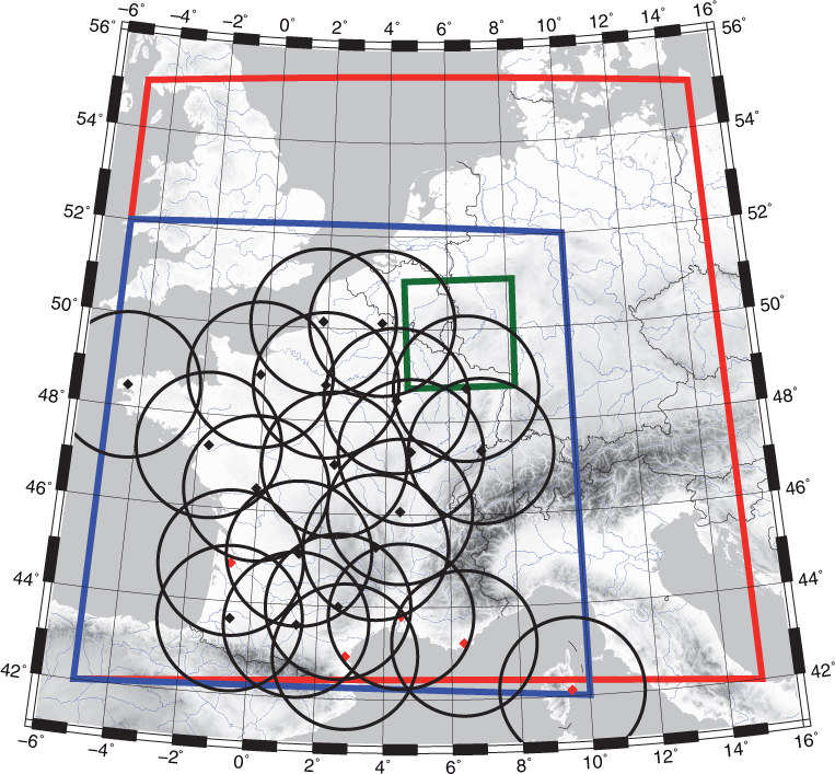
Fig. 2
Coverage of the different radar systems applied in the WRF experiment. The radar circles of the French systems have a radius of approx. 160 km; the red dots represent S-band radar systems and the black dots C-band radars. The red frame marks the verification domain for the qualitative verification, the green frame shows the small verification domain centred over Luxembourg and the blue frame marks the verification domain for the investigation of the performance of the radar data assimilation.
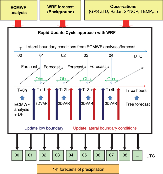
Fig. 3
Sketch illustrating the WRF QPE approach.
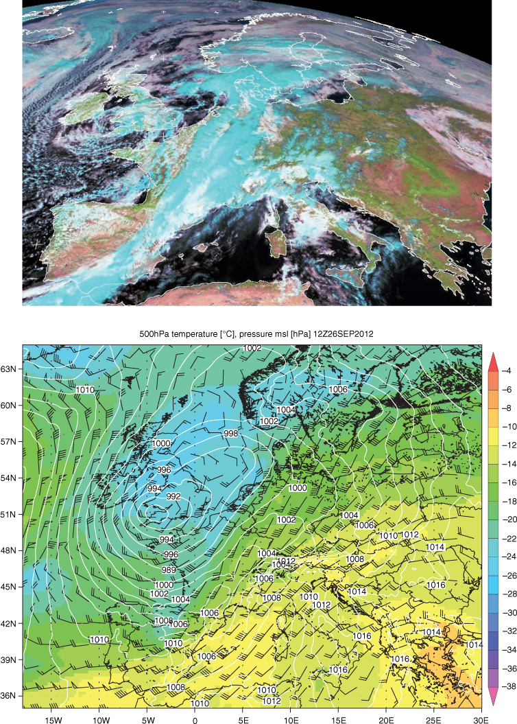
Fig. 4
Synoptic situation at 12 UTC, 26 September 2012. Top: ‘Natural colour’ composite image of the Meteosat Satellite (Source: NERC satellite receiving station, Dundee University, from http://www.sat.dundee.ac.uk/). Clouds containing ice particles are coloured in cyan. Bottom: ECMWF analysis showing the 500 hPa temperature (°C) (colour) and wind field as well as the mean sea level pressure (hPa) (white contours).
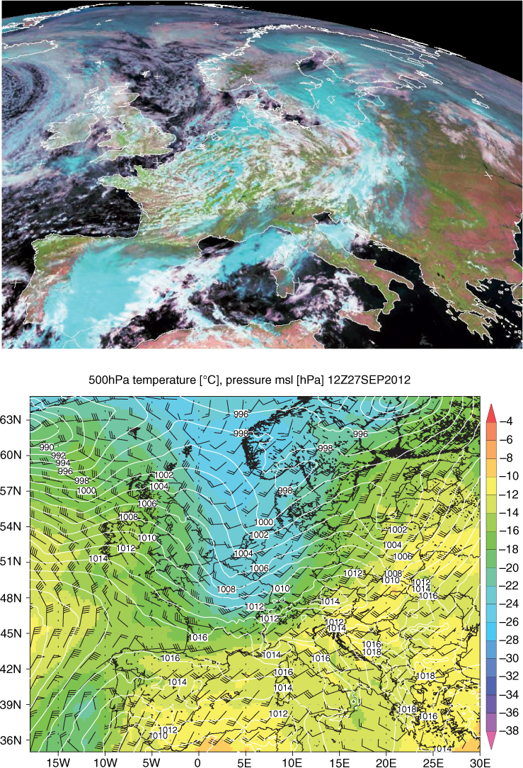
Fig. 5
Same as Fig. 5, but for 12 UTC, 27 September 2012.

Fig. 6
Comparison of the maximum reflectivity (dBZ) of the WRF CONTROL simulation (top left), the merged reflectivity composite of Météo France and DWD (top right) (areas not covered by radar in grey), the ASSIM_NORAD simulation (bottom left) and the ASSIM_ALL simulation (bottom right) for 02 UTC, 26 September 2012.
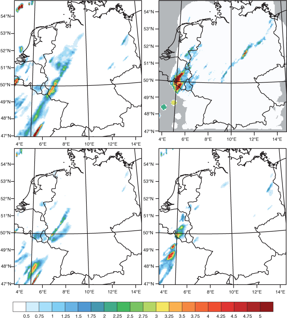
Fig. 7
Comparison of the hourly accumulated precipitation (mm/h) of the WRF CONTROL simulation (upper left), the DWD RADOLAN RW product (upper right), the ASSIM_NORAD simulation (lower left) and the ASSIM_ALL simulation (lower right) for 02 UTC, 26 September 2012.
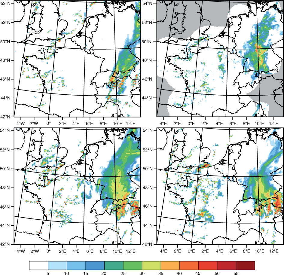
Fig. 8
Same as Fig. 6, but for 01 UTC, 27 September 2012.
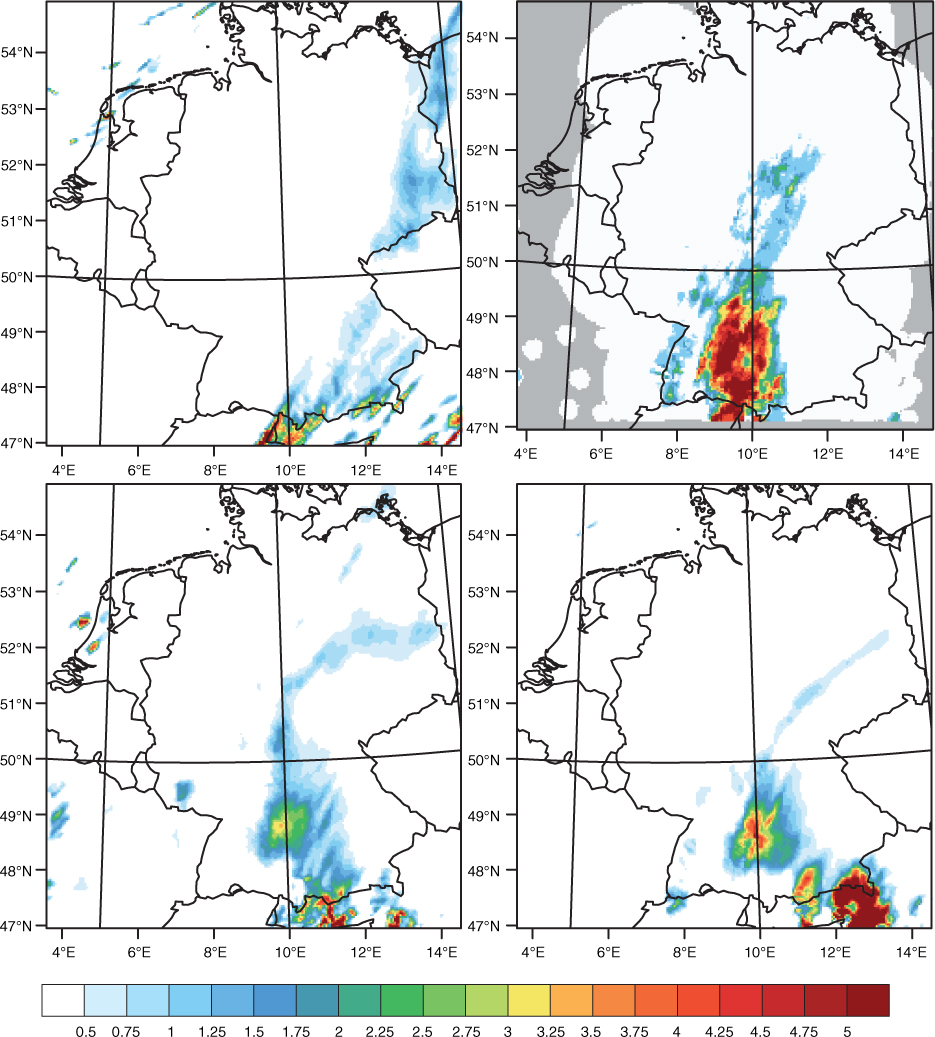
Fig. 9
Same as Fig. 7, but for 01Z, 27 September 2012.
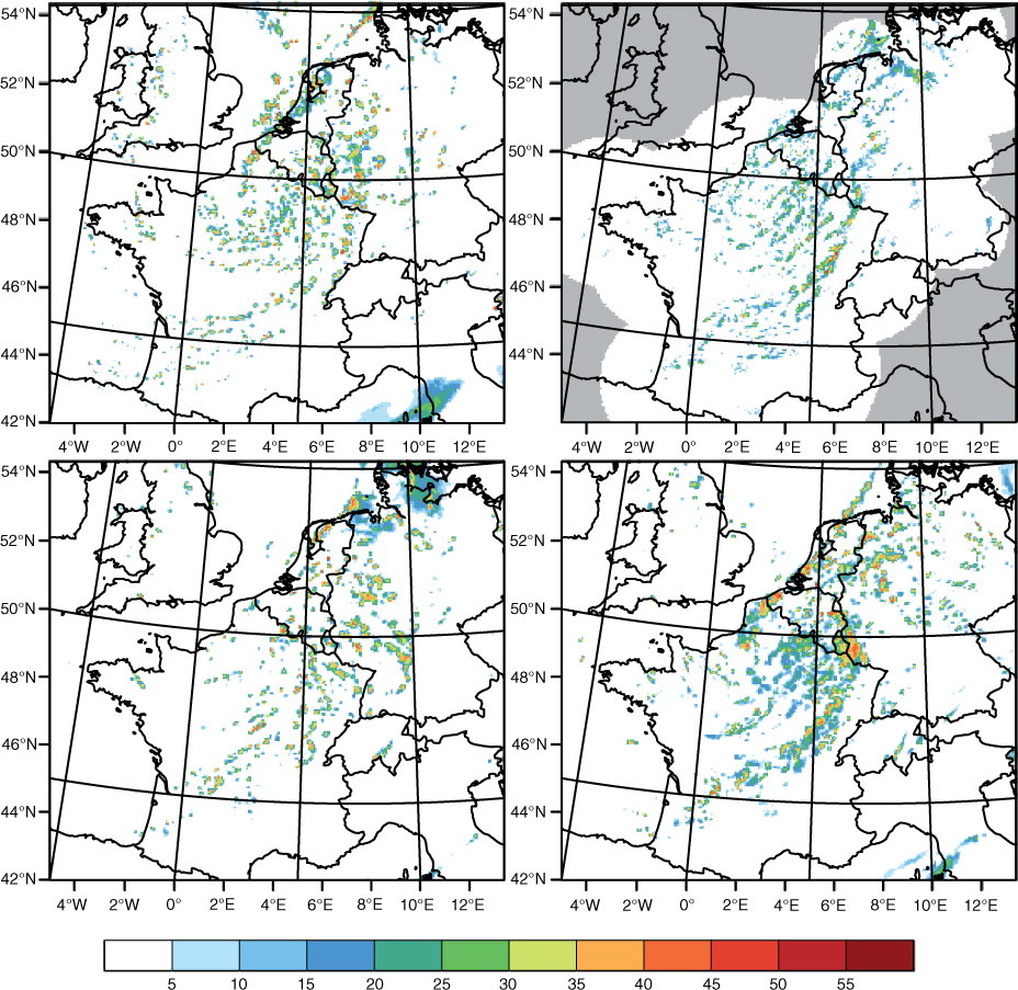
Fig. 10
Same as Fig. 6, but for 12 UTC, 27 September 2012.
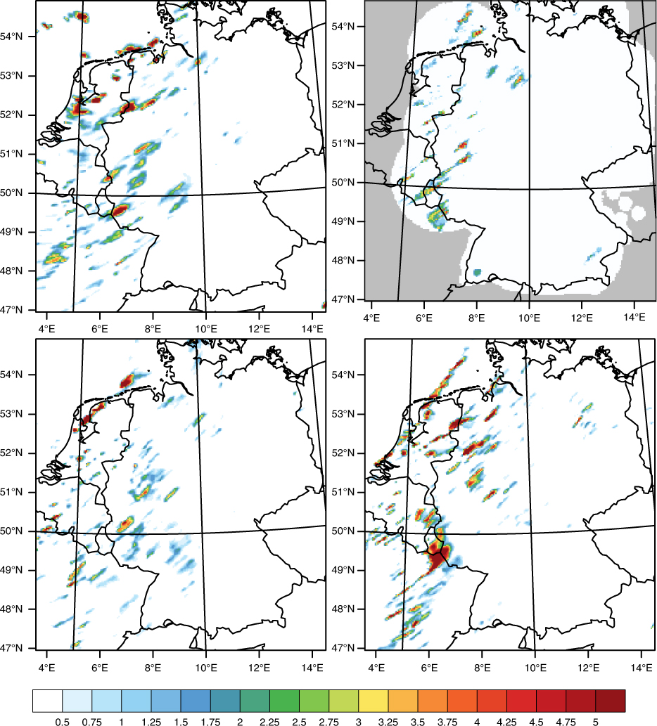
Fig. 11
Same as Fig. 7 but for 12 UTC, 27 September 2012.
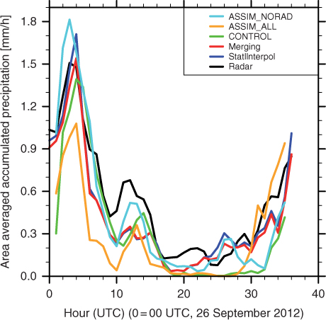
Fig. 12
Time series of hourly accumulated and area averaged precipitation amounts (mm/h) from 00 UTC, 26 September 2012 until 12 UTC, 27 September 2012 for spatially interpolated rain gauge data (blue), precipitation derived from Wideumont radar data (black), a merged product of the two (red) and the three model simulations CONTROL (green), ASSIM_NORAD (cyan) and ASSIM_ALL (orange).
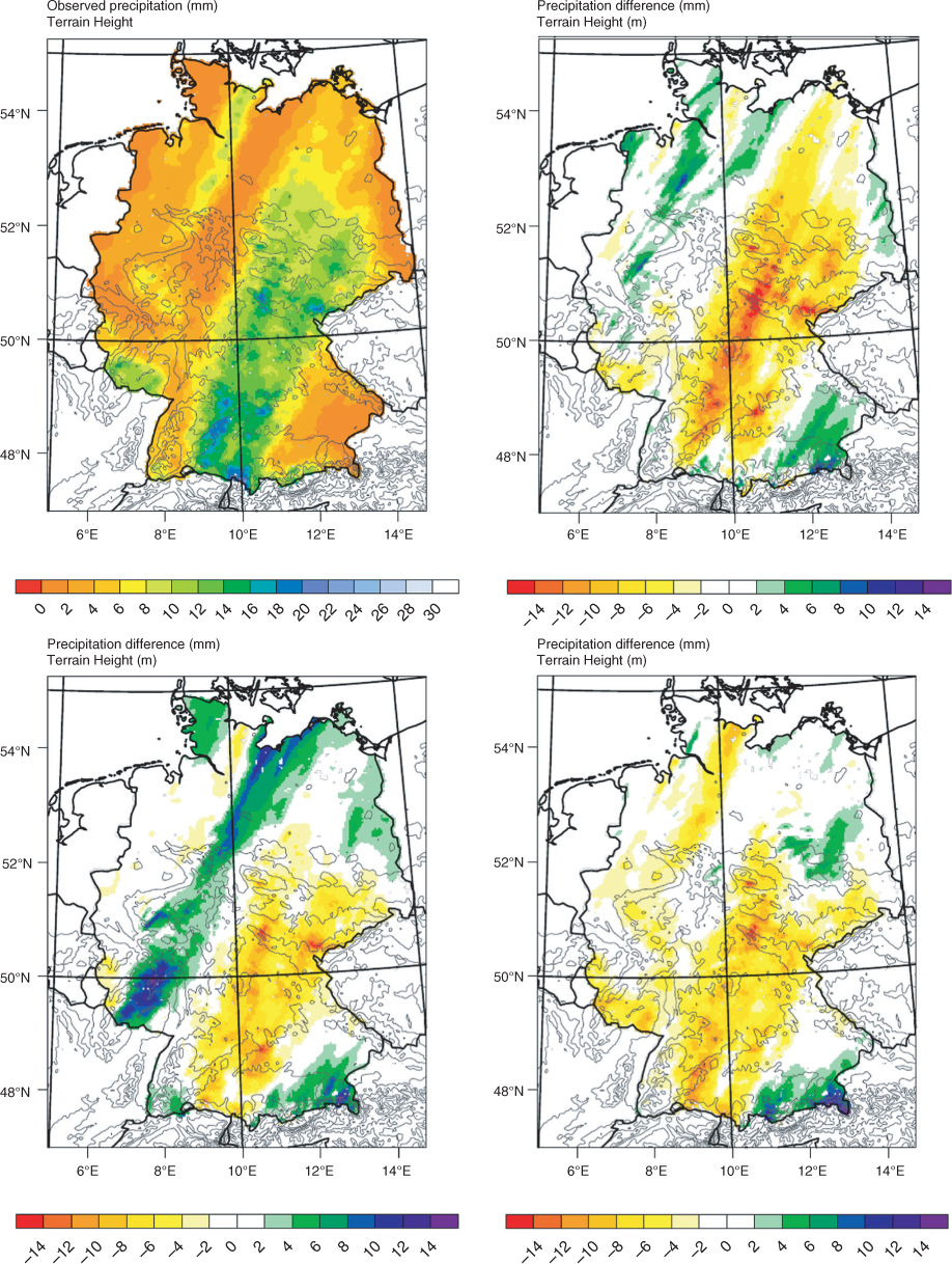
Fig. 13
Comparison of the 24-hourly accumulated precipitation from 06 UTC, 26 September 2012 until 06 UTC, 27 September 2012 of REGNIE (upper left) and MODEL – REGNIE differences of CONTROL (upper right), ASSIM_NORAD (lower left) and ASSIM_ALL (lower right). Contour lines indicate orography.
Table 2. Verification scores derived from the comparison of the 24-hourly accumulated precipitation (06 UTC, 26 September 2012 until 06 UTC, 27 September 2012) of the model simulations and the DWD REGNIE product
BIAS (mm)−2.18−0.28−2.19RMSE (mm)5.024.54.22Mean correlation0.20.290.56Equitable threat score1 mm/24 h0.10.120.125 mm/24 h0.070.170.2910 mm/24 h0.070.060.06Frequency bias1 mm/24 h0.991.060.915 mm/24 h0.581.160.6110 mm/24 h0.180.380.3
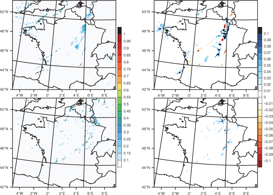
Fig. 14
Comparison of rain water mixing ratio (g/kg) of the 1-hour forecast (First Guess) (left column) and the Analysis – First Guess difference (right column) for 02 UTC, 26 September 2012 (upper line) and 12 UTC, 27 September 2012 (lower line) at model level 14 (approximately 1300 m above ground level).

Fig. 15
Same as Fig. 14, but for cloud water mixing ratio (g/kg).
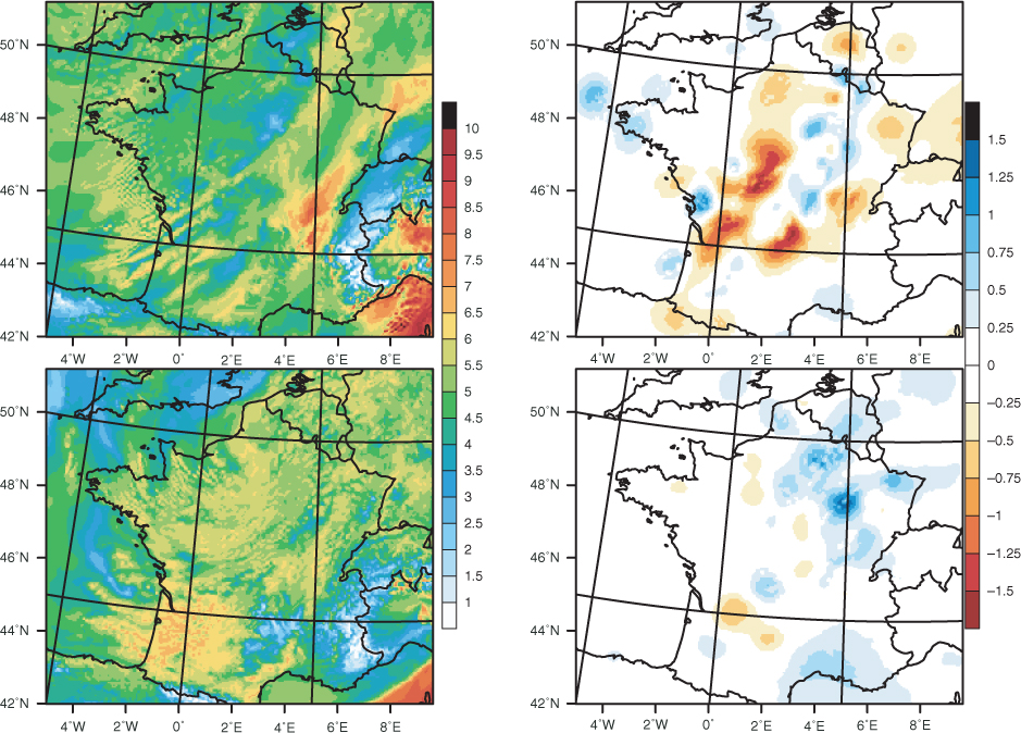
Fig. 16
Same as Fig. 14, but for water vapour mixing ratio (g/kg).
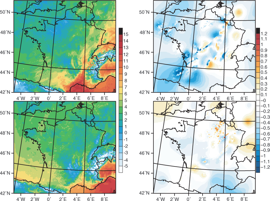
Fig. 17
Same as Fig. 14, but for temperature (°C).