
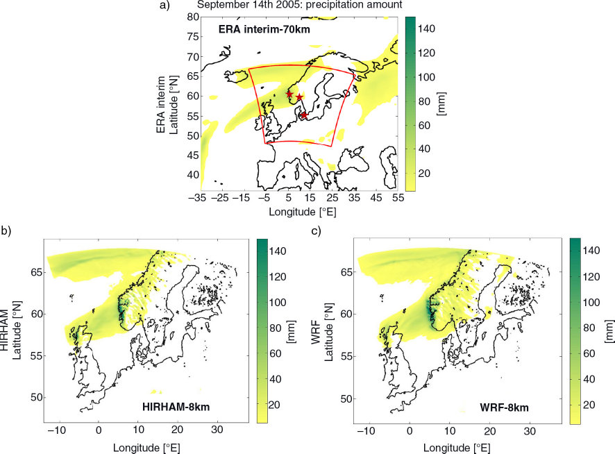
Fig. 1.
(a) 24-hour precipitation amount in mm on 14 September 2005 as represented in the ERA interim data product. The red box indicates the domain used to perform dynamical downscaling. The locations of Bergen, Oslo and Copenhagen are indicated with red stars. The maps below show the same variable as simulated in the RCMs: (b) HIRHAM5 and (c) WRF.
Table 1.
Chosen physical options within the two regional climate model simulations
Table 2. Seasonal biases of temperature and wet-day precipitation
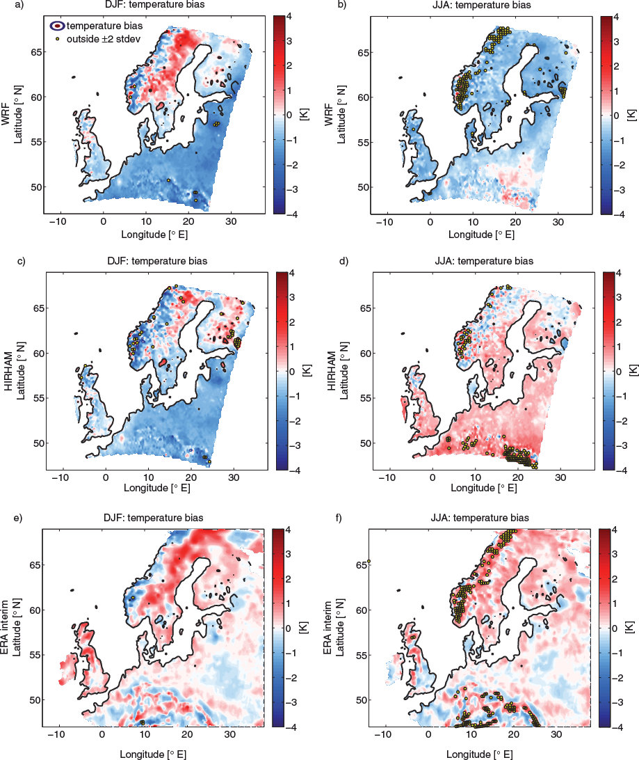
Fig. 2.
Biases of seasonal temperature in K (simulation minus E-OBS data) in the WRF simulation for (a) winter and (b) summer season; (c, d) for the HIRHAM5 simulation; and (e, f) for ERA interim. Model data is re-projected bilinearly to the E-OBS 0.22° rotated grid. Yellow dots indicate grid points where the model biases lie outside an interval of ±2 standard error which is given within the E-OBS data set.
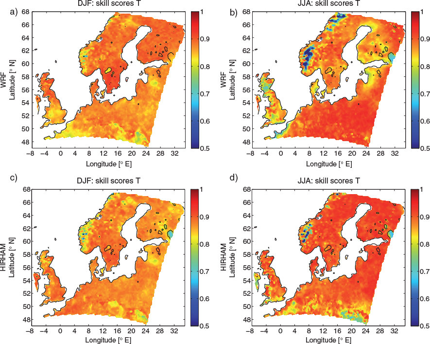
Fig. 3.
Skill scores for daily mean temperature, T, for the WRF simulation for the seasons (a) winter and (b) summer; (c, d) as simulated in HIRHAM5. The skill score is dimensionless and ranges from 0 to 1, where 1 is a perfect match between the observed and modelled distributions. The colour bar ranges from 0.5 to 1 to make regional differences more visible
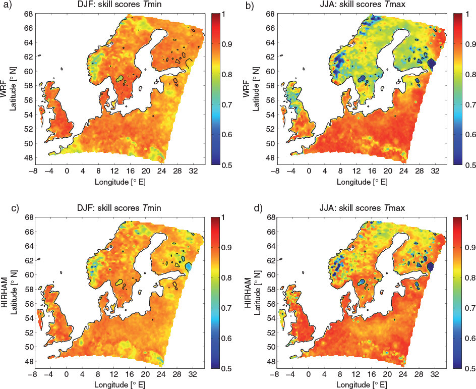
Fig. 4.
As in Fig. 3 for extreme temperatures. (a) winter minimum temperature, Tmin, in WRF and (c) Tmin in HIRHAM5. (b) and (d) represent the skill scores in summer maximum temperatures, Tmax, in WRF and HIRHAM5, respectively.
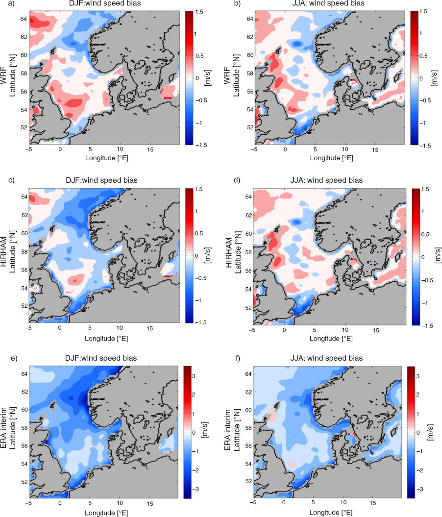
Fig. 5.
Biases of wind speed in m s−1 (simulation minus Qscat) in (a) and (b) WRF; (c, d) HIRHAM; and (e, f) ERA interim. The winter season is shown in the left column and the summer season in the right column. Grey areas indicate no data.
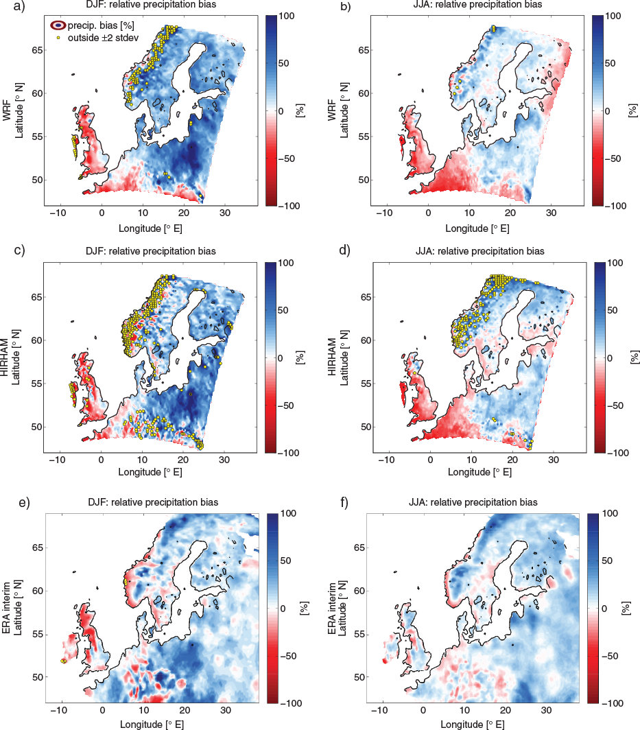
Fig. 6.
Relative precipitation bias, . 100% in the WRF simulation for (a) winter and (b) summer season; (c, d) for the HIRHAM5 simulation; and (e, f) for ERA interim. Yellow dots indicate grid points where the model biases lie outside an interval of ±2 standard error which is given within the E-OBS data set. The absolute error ranges between ±3 mm day−1.
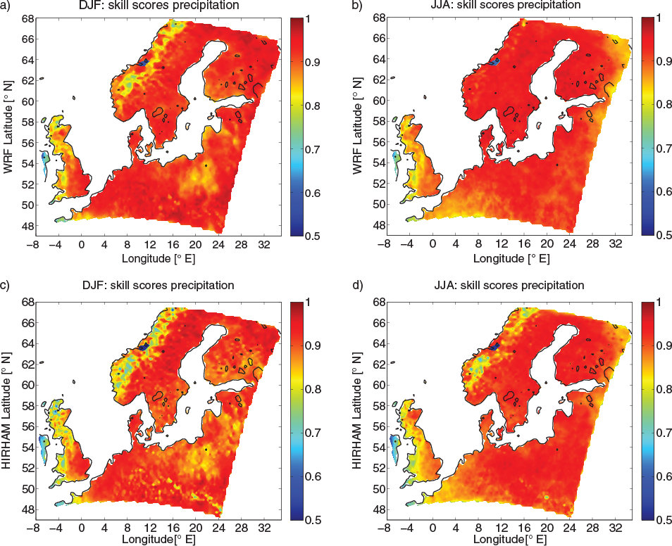
Fig. 7.
As in Fig. 3 for daily mean precipitation amounts for the WRF simulation for the seasons (a) winter and (b) summer; c, d) as simulated in HIRHAM5.
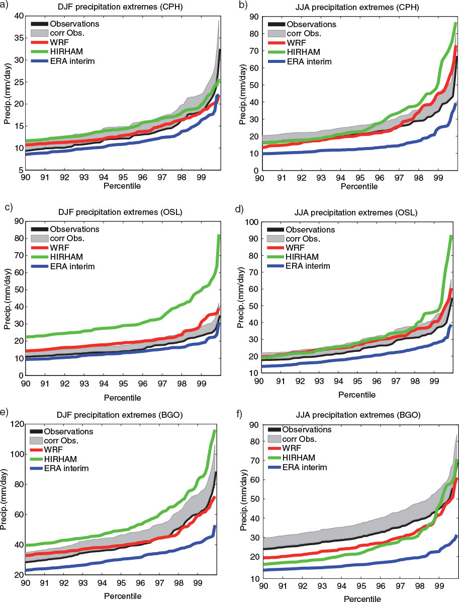
Fig. 8.
90–99.9 percentiles for extreme precipitation in mm day−1 for (a) and (b) Copenhagen; (c, d) Oslo; and (e, f) Bergen. Corresponding model data was retrieved with the nearest-neighbour method for the single locations. The subfigures in the left column represent wintertime (DJF) extreme precipitation. In the right column, summertime (JJA) extreme precipitation is shown. An assumed observational undercatch of 20% is illustrated with a grey band.
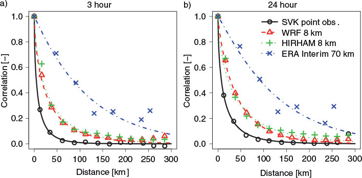
Fig. 9.
Spatio-temporal correlation structure of observed (SVK), ERA interim (70 km) and downscaled (8 km) mean intensities of extreme precipitation for 3 hour (a) and 24 hour (b) duration. To highlight the tendencies, an exponential function is used for fitting by using the least-square method.
Table 3.
Estimated e-folding distances in km of extreme precipitation for the duration of 3 hours and 24 hours
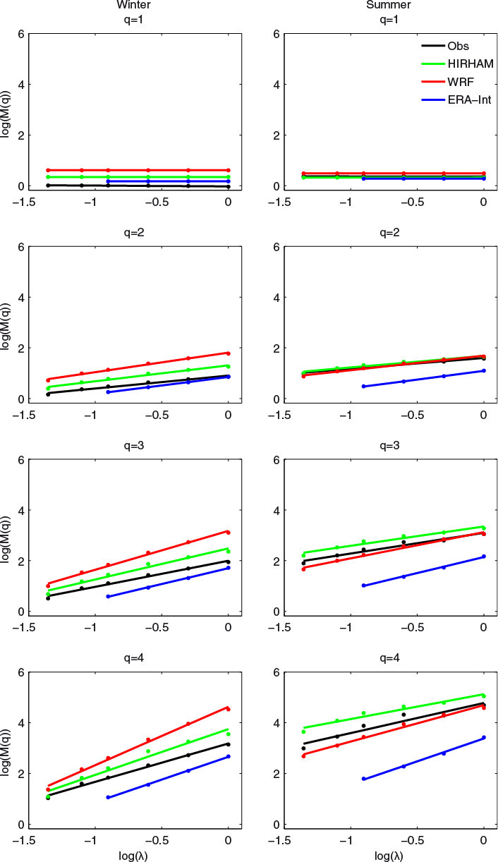
Fig. 10.
Moment scaling relationships for the observed and simulated precipitation in Copenhagen during winter (left) and summer (right). q = 1 mean; q = 2 standard deviation; q = 3 skewness and q = 4 kurtosis. The abscissa represents the different temporal aggregations.
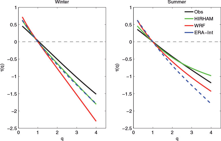
Fig. 11.
Summary of Fig. 10 with the different slopes τ as a function of the statistical moments q.