
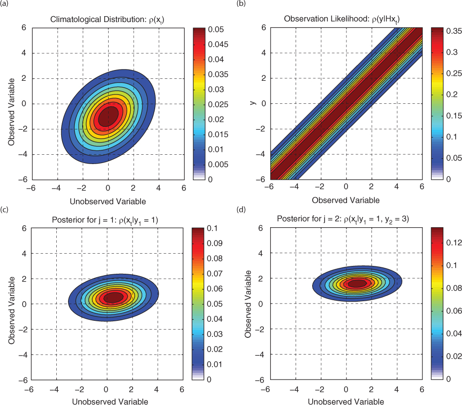
Fig. 1
Data assimilation on the high-resolution (true) attractor. (a) High-resolution climatological distribution, (b) high-resolution observation likelihood, (c) high-resolution posterior for j=1 and (d) high-resolution posterior for j=2.
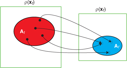
Fig. 2
The attractors and their map. The two green squares represent the domain of the true states (large square) and the forecast states (small square). The region for which is denoted as the red (blue) shaded region. An example of the function in eq. (4) is denoted by the arrows, which travel from states in 𝔸 t denoted by filled circles to states in 𝔸 f denoted by open circles. Note that multiple states in 𝔸 t may map to the same point in 𝔸 f . We will show that this results in an error of representation.
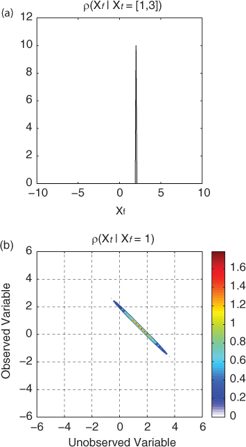
Fig. 3
The conversion densities. (a) The conversion density describing the distribution of forecast states given a state on the true attractor (), and (b) the conversion density describing the distribution of true states given a state on the forecast attractor (x f =1).

Fig. 4
Data assimilation on the low-resolution (forecast) attractor. The low-resolution (a) observation likelihood and (b) climatological and posterior distributions for j=1 and 2.
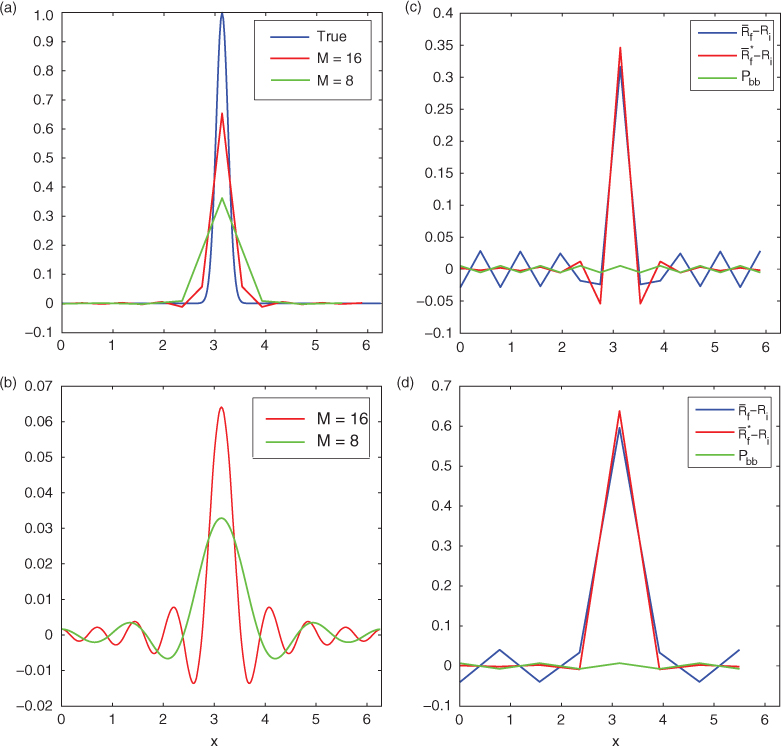
Fig. 5
Pure spectral truncation. (a) Three one-point prior covariance functions: blue is the high-resolution (true) covariance model, red is the M=16 low-resolution (forecast) covariance model and green is the M=8 low-resolution (forecast) covariance model. (b) One column of the smoother matrix [eq. (62)] for M=16 (red) and M=8 (green). (c, d) The main components of the theory for M=16 and M=8, respectively: blue is the representation error covariance (), red is the effective representation error covariance () and green is the bias covariance matrix (P bb ).
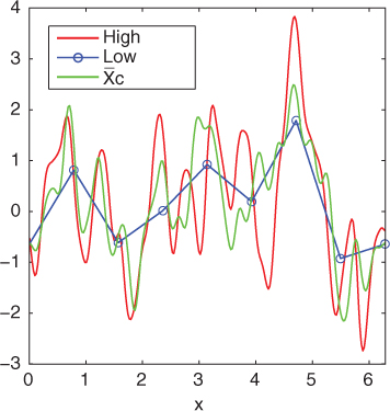
Fig. 6
Example high-resolution state, low-resolution state (M=8) and mean of the conversion density, which is labelled above as the ‘best estimate’. The low-resolution state is defined only at the grid-points denoted by the open circles.
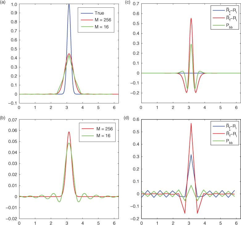
Fig. 7
Gaussian Smoothing. (a) Three one-point prior covariance functions: blue is the high-resolution (true) covariance model, red is the M=256 low-resolution (forecast) covariance model and green is the M=16 low-resolution (forecast) covariance model. (b) One column of the smoother matrix for M=256 (red) and M=16 (green). (c, d)The main components of the theory for M=256 and M=16, respectively: blue is the representation error covariance (), red is the effective representation error covariance () and green is the bias covariance matrix (P bb ).