
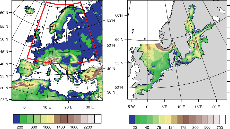
Fig. 1
RCA4 domain and topography (the red square is the domain of the river routing model CaMa-Flood) (left) and the ocean model domain and bathymetry (right) (unit: meter).
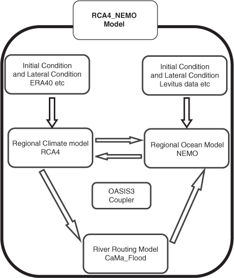
Fig. 2
Schematic diagram of the coupled model system (The sea ice model LIM3 is part of NEMO and not coupled via OASIS3).
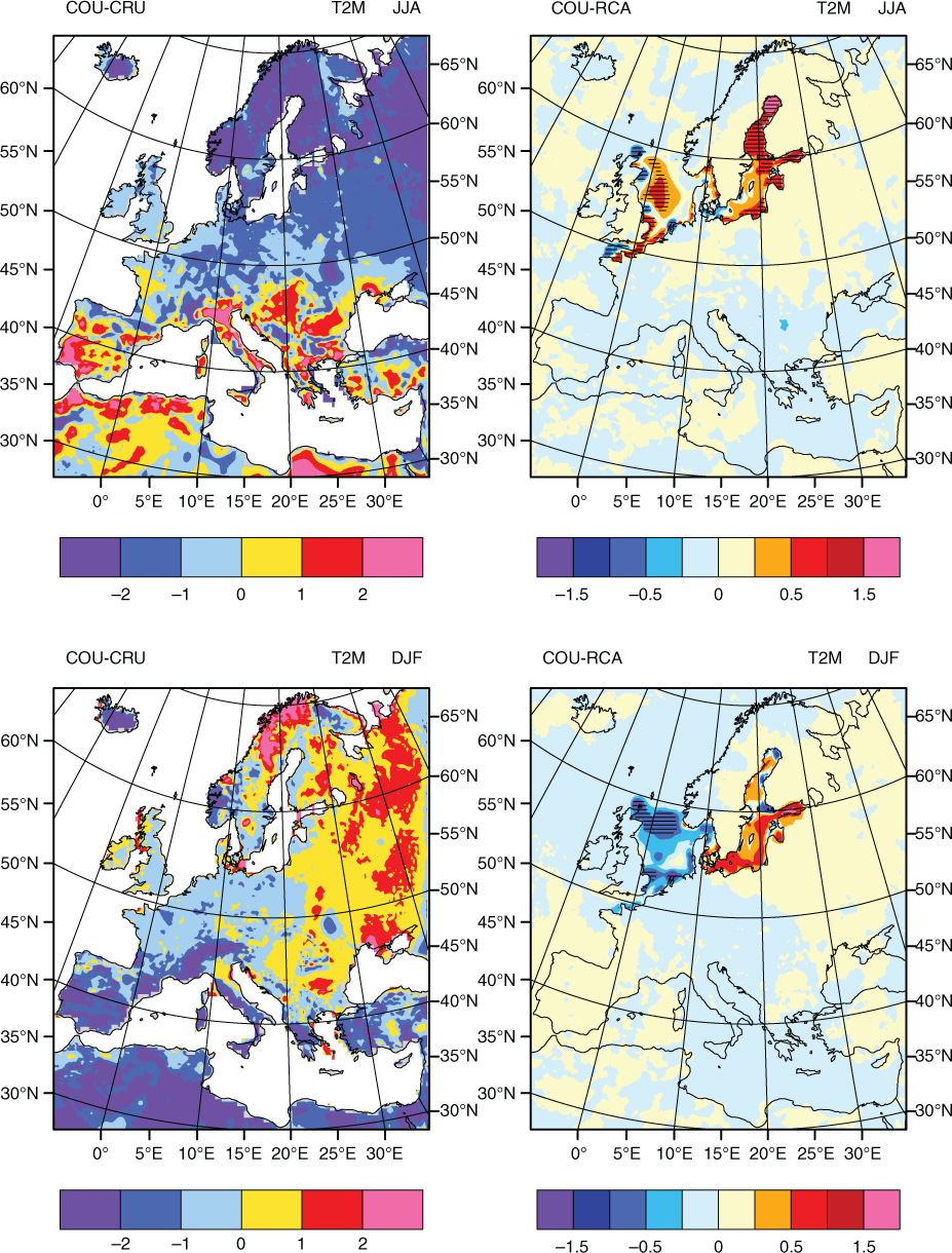
Fig. 3
Seasonal mean 2 m temperature (T2M) differences between the coupled run and observations (COU-CRU), and between the coupled run and the uncoupled atmosphere run (COU-RCA) for summer (JJA, top panel) and winter (DJF, bottom panel) (unit: K). Hatching indicates differences with significance level exceeding 95%.
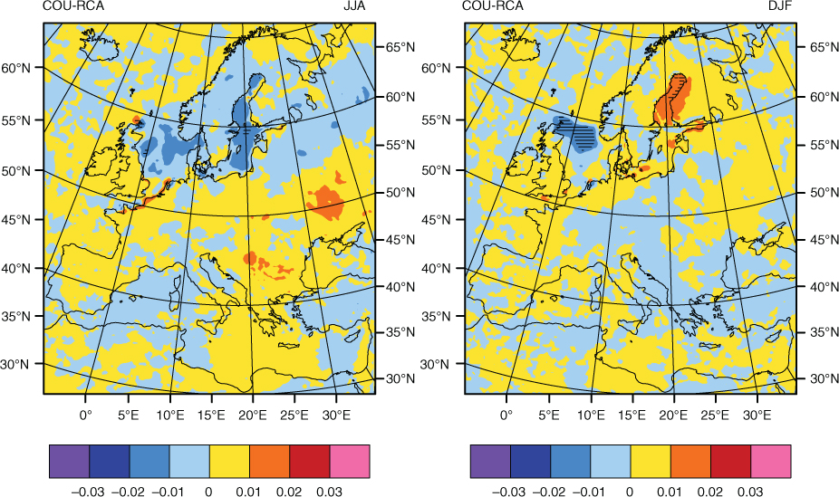
Fig. 4
Seasonal mean differences of total cloud cover between the coupled run and the uncoupled atmosphere run (COU-RCA) for summer (JJA, left) and winter (DJF, right) (unit: fraction). Hatching indicates differences with significance level exceeding 95%.
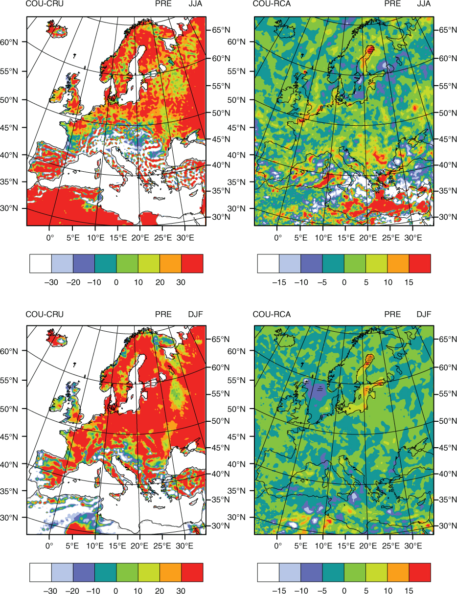
Fig. 5
Seasonal mean precipitation (PRE) relative differences (%) between the coupled run and observations (COU-CRU), and between the coupled run and the uncoupled atmosphere run (COU-RCA) for summer (JJA, top panel) and winter (DJF, bottom panel). Hatching indicates differences with significance level exceeding 95%.
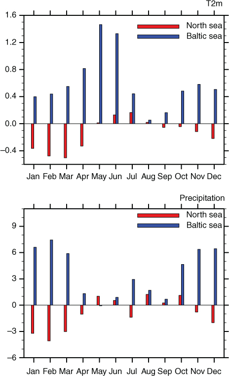
Fig. 6
2 m temperature (top, unit: K) and precipitation (bottom, unit:%) differences between the coupled run and the uncoupled atmosphere run in the North Sea and Baltic Sea.
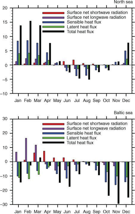
Fig. 7
Heat flux differences between the coupled run and the uncoupled atmosphere run in the North Sea (top) and Baltic Sea (bottom) (unit: W/m2). Positive values indicate fluxes into the ocean.
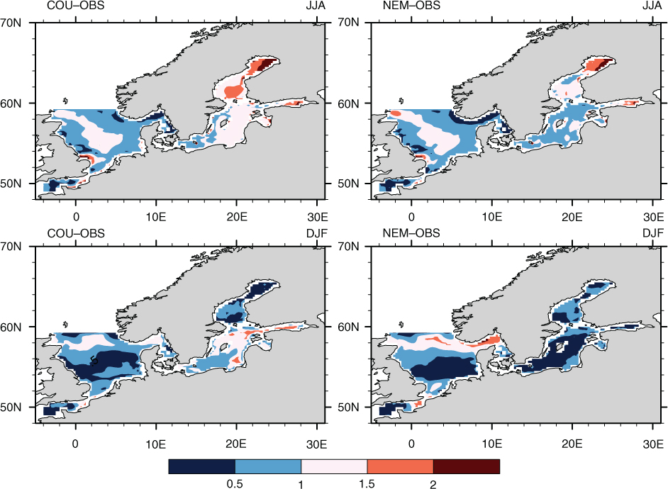
Fig. 8
RMSE of SST between the coupled model and observations (COU-OBS, left) and between the uncoupled ocean model and observations (NEM-OBS, right) for summer (JJA, top panel) and winter (DJF, bottom panel) (unit: K).
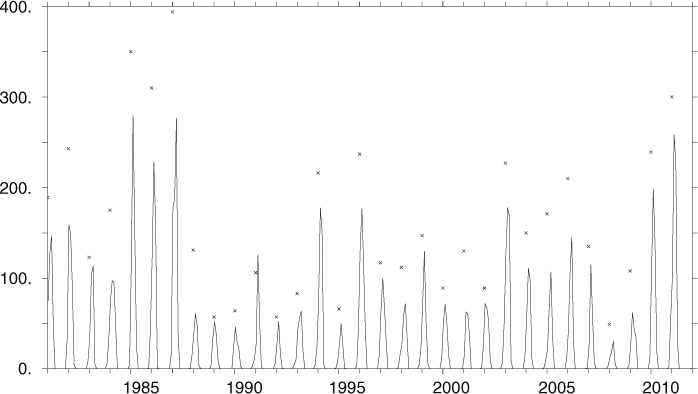
Fig. 9
Monthly mean Baltic Sea ice extent from the coupled simulation (black line) and observed maximum ice extent (black crosses) (unit: 109 m2).
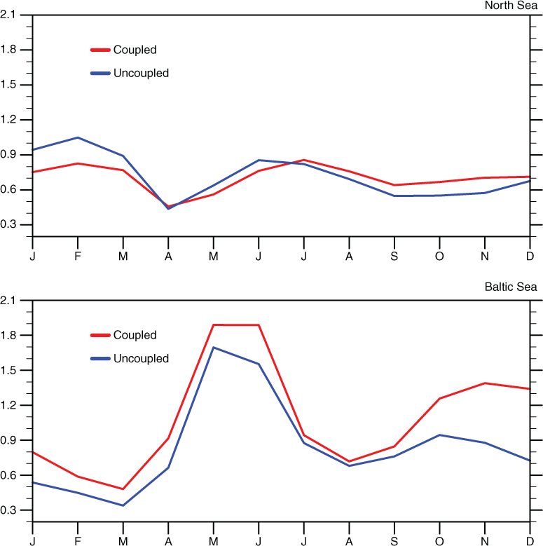
Fig. 10
Spatial averaged RMSE of SST for the coupled run and uncoupled atmosphere run in the North Sea (top panel) and Baltic Sea (bottom panel) (unit: K).
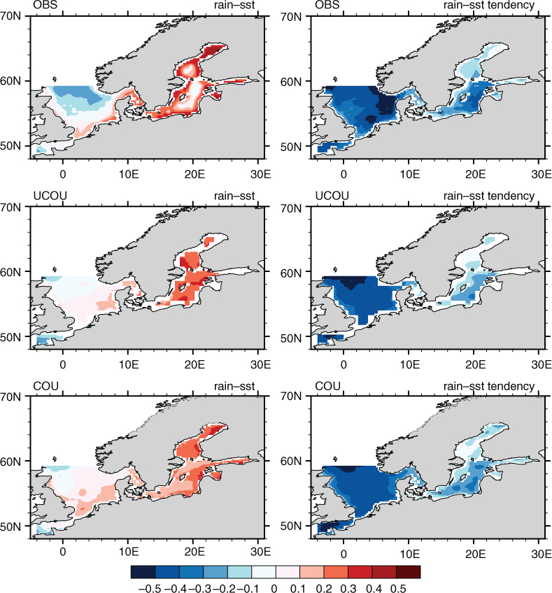
Fig. 11
Top panel: correlation between precipitation and SST (left) and correlation between precipitation and SST tendency (right) for observations (OBS). Middle panel: as top panel except for uncoupled atmosphere run (UCOU). Bottom panel: as top panel except for the coupled run (COU).
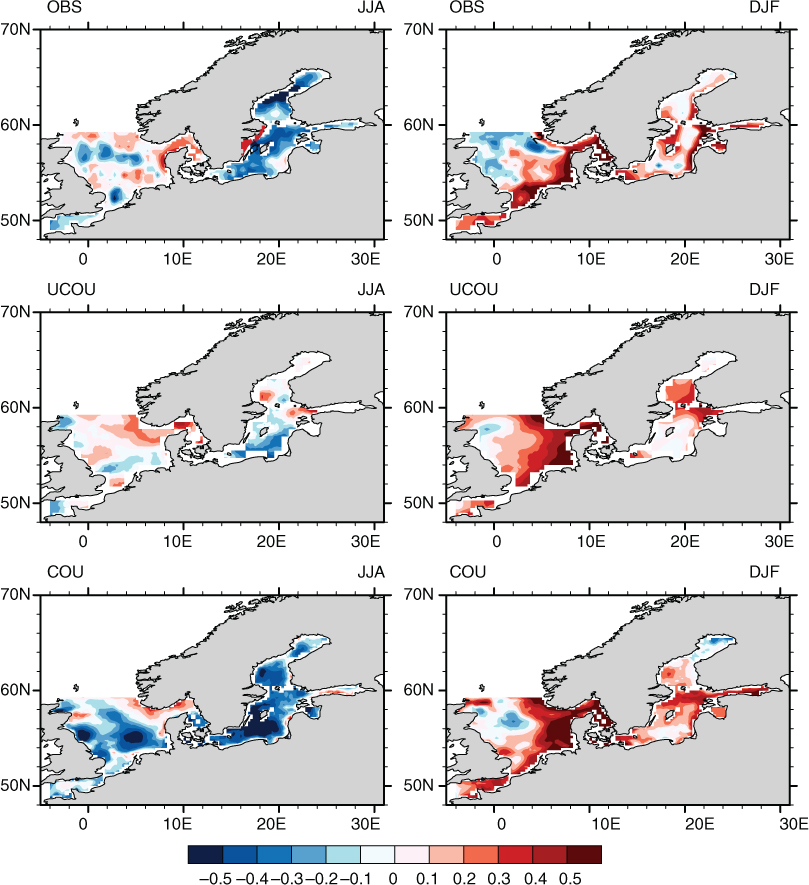
Fig. 12
Top panel: precipitation-SST correlation for observation (OBS) in summer (JJA, left column) and winter (DJF, right column). Middle panel: as top panel except for the uncoupled atmosphere simulation (UCOU). Bottom panel: as the top panel except for the coupled simulation (COU).
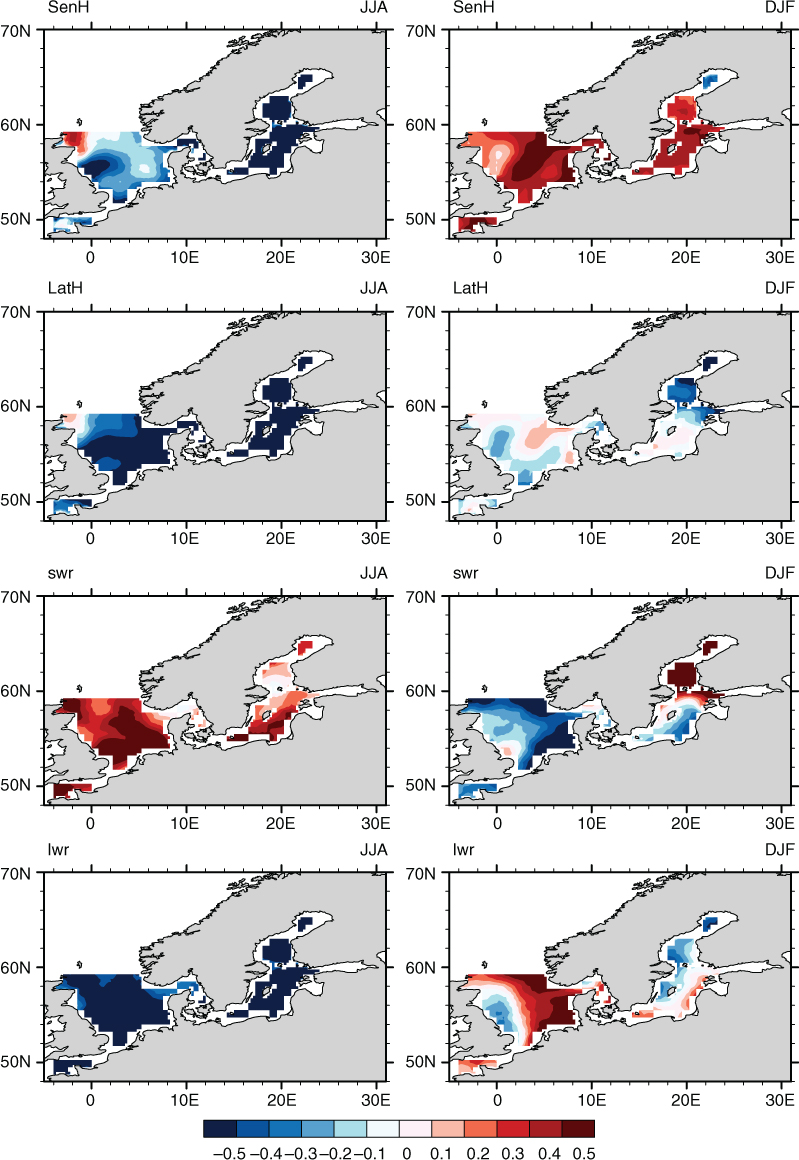
Fig. 13
Correlations between sensible heat flux (SenH), latent heat flux (LatH), short wave radiation (swr), long wave radiation (lwr) and SST (from top to bottom) in Summer (JJA, left column) and winter (DJF, right column) for the uncoupled atmosphere run.
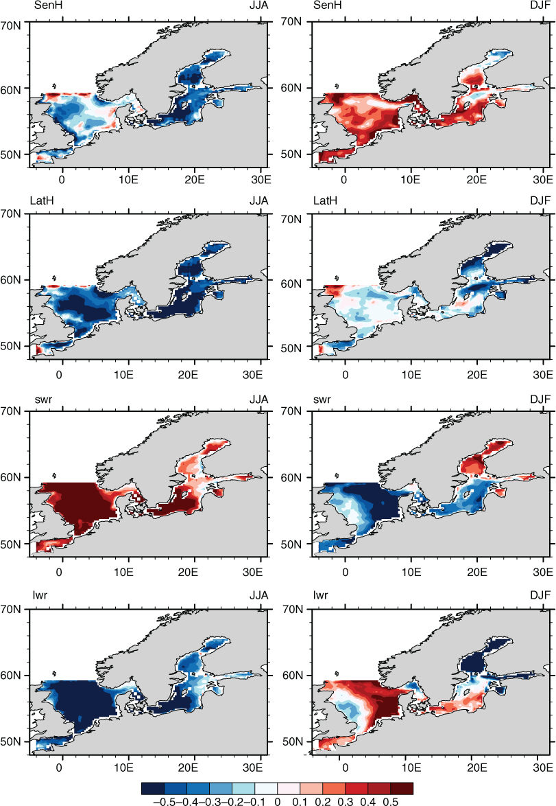
Fig. 14
Similar to Fig. 13 except for the coupled run.
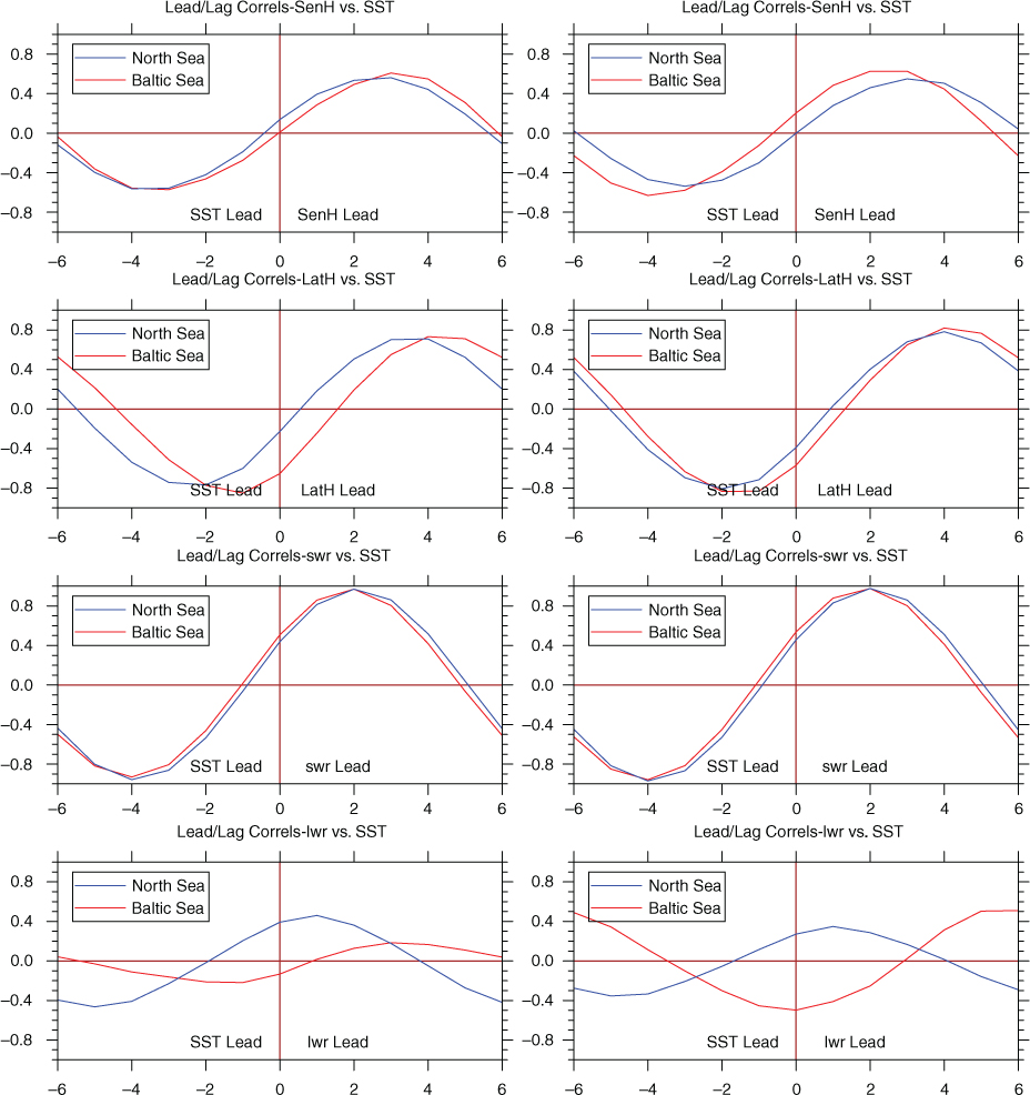
Fig. 15
Lead/lag correlations between sensible heat flux (SenH), latent heat flux (LatH), short wave radiation (swr), long wave radiation (lwr) and SST (from top to bottom) for the uncoupled atmosphere run (left column) and the coupled run (right column) (X-axis: month).