
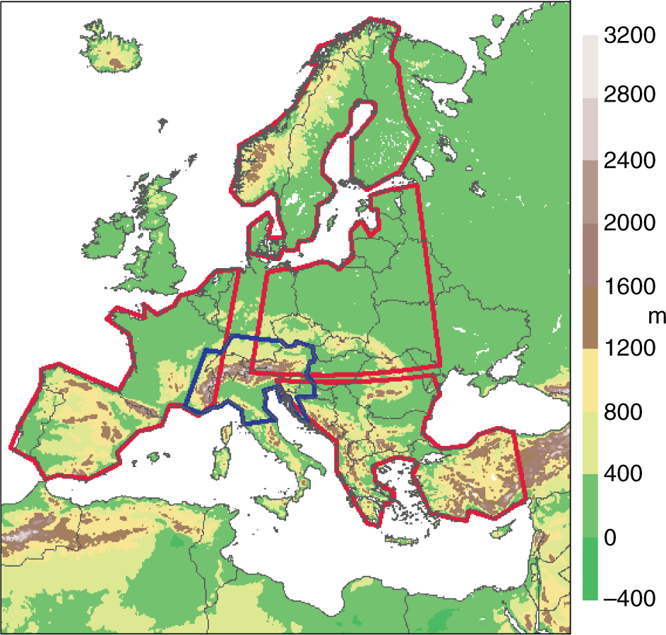
Fig. 1
Model domain and topography from HCLIM6. European subareas analysed in Sections 4.1 and 4.2 are marked in red: North Europe, West Europe, East Europe and South-East Europe. Blue marked area represents the Alps region, used in Section 4.5.
Table 1. Vertical model levels converted to pressure (hPa), with a surface pressure of 1013.25 hPa
110214494181823022470428323512349243845471245144485859225535458706114265564688271352757647893815728596489049179296164991510202306355092511224316555193412246326735294413269336915395314291347095496115314357265597016337367455697817359377595798618382387745899419404397905910022042640804601009
Table 2. Evaluation data used in the study
E-OBSGridded obs.
Version 7.0T2m, Pr0.25°Haylock et al. (2008)CRUGridded obs.
Version TS 3.1Clt0.5°Harris et al. (2013)ERA-InterimECMWF
ReanalysisSLP, pr, clt, SWd,
LWd, R n , LH, SH0.79°Dee et al. (2011)PPSCM-SAF Polar
Platform System clt, LWd0.25°2009)MSGCM-SAF MeteosatSWd0.25°2009)Second GenerationMetNoGridded obs.Pr1 km2005)NorwayPTHBVGridded obs.T2m, Pr4 km2002)RhiresDGridded obs.Pr2.2 kmMeteoSwiss (2010) SwitzerlandEURO4M-APGDGridded obs.Pr5 kmIsotta et al. (2013) Alpine regionTabsDGridded obs.T2m2.2 kmMeteoSwiss (2011) SwitzerlandREGNIEGridded obs.Pr1 kmRauthe et al. (2013) GermanySAFRANReanalysis
FranceT2m, Pr8 km2008), Vidal et al. (2010)Spain02Gridded obs.
SpainT2m, Pr0.2°Herrera et al. (2012)BSRNGround-based obs.SWdPointKönig-Langlo et al. (2013)
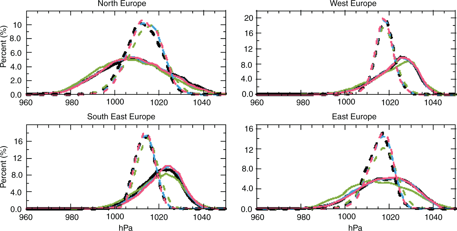
Fig. 2
Winter (solid lines) and summer (dashed) PDFs of sea level pressure for HCLIM6 (red), HCLIM15 (blue), RCA4 (green) and ERA-I (black) for four European subregions. Note that ERA-I can be somewhat hidden in some regions because it coincides with HCLIM6 and HCLIM15.
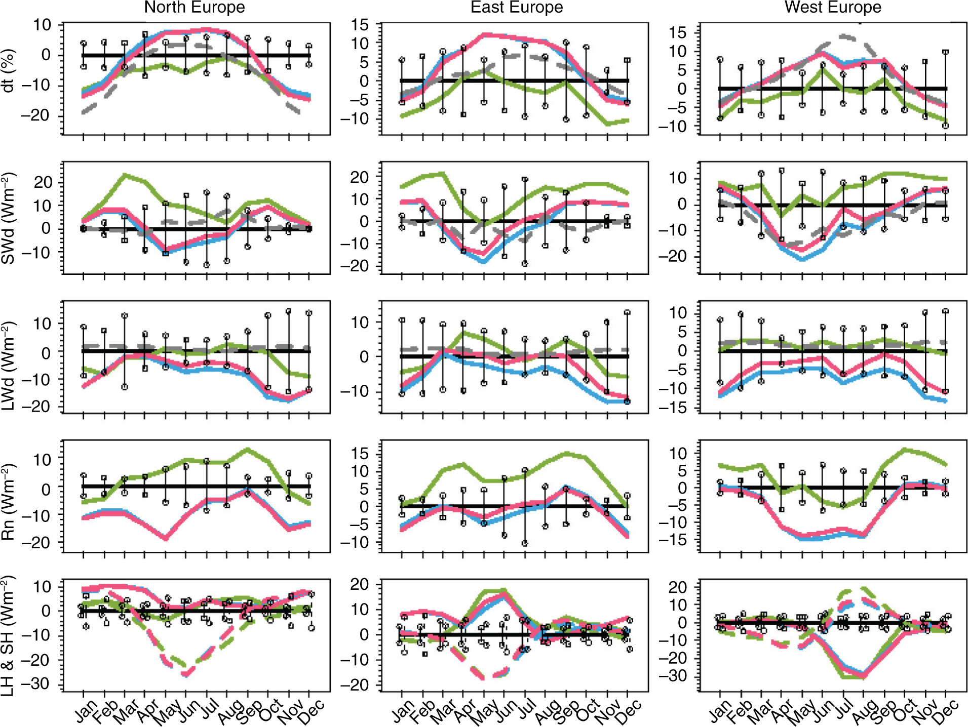
Fig. 3
Annual cycle with reference to ERA-I (black) of (top to bottom) cloud fraction (clt), downwelling solar radiation (SWd), downwelling thermal radiation (LWd), surface net radiation budget (R n ) and latent (solid) and sensible (dashed) surface heat fluxes. HCLIM6 (red), HCLIM15 (blue), and RCA4 (green). Positive LWd/SWd means too much radiation downwelling to the surface and negative means too little compared to ERA-I. The vertical bars represent ±1 standard deviation based on the 10 yr of monthly values from ERA-I. The grey dashed line is the satellite product CM-SAF, the PPS product for clt and LWd and the MSG product for SWd.
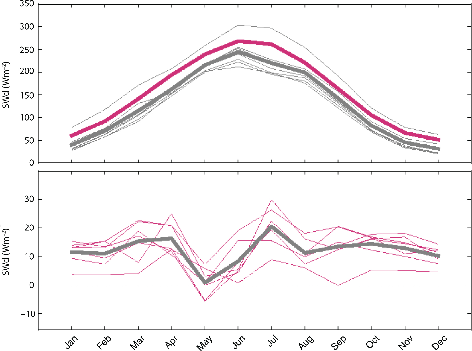
Fig. 4
Annual cycle of downwelling solar radiation from seven measuring towers from the BSRN dataset. Top figure shows absolute values from BSRN and HCLIM6. Thin grey lines are individual BSRN observations, and the thick grey and red lines are the mean values from BSRN and HCLIM, respectively. Bottom figure shows HCLIM6 anomalies (red lines) with reference to corresponding BSRN station and the mean bias (thick grey line). HCLIM6 values are taken from the grid cell nearest the respective observation site.
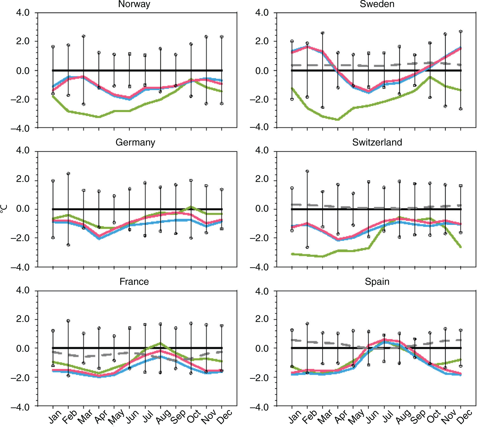
Fig. 5
Annual cycle for 6 European subregions with reference to E-OBS (black) of 2 m temperature, HCLIM6 (red), HCLIM15 (blue) and RCA (green). The vertical bars represent ±1 standard deviation based on the 10 yr of monthly values from E-OBS. The grey dashed lines are high-resolution observations (cf. Table 2).
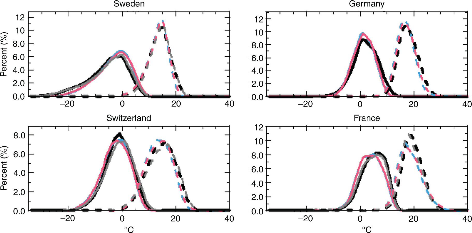
Fig. 6
PDF of winter (DJF, solid lines) and summer (JJA, dashed lines) 2 m temperature. HCLIM6 (red), HCLIM15 (blue) and E-OBS (black). The grey lines are high-resolution observations: PTHBV (Sweden), TabsD (Switzerland) and SAFRAN (France).
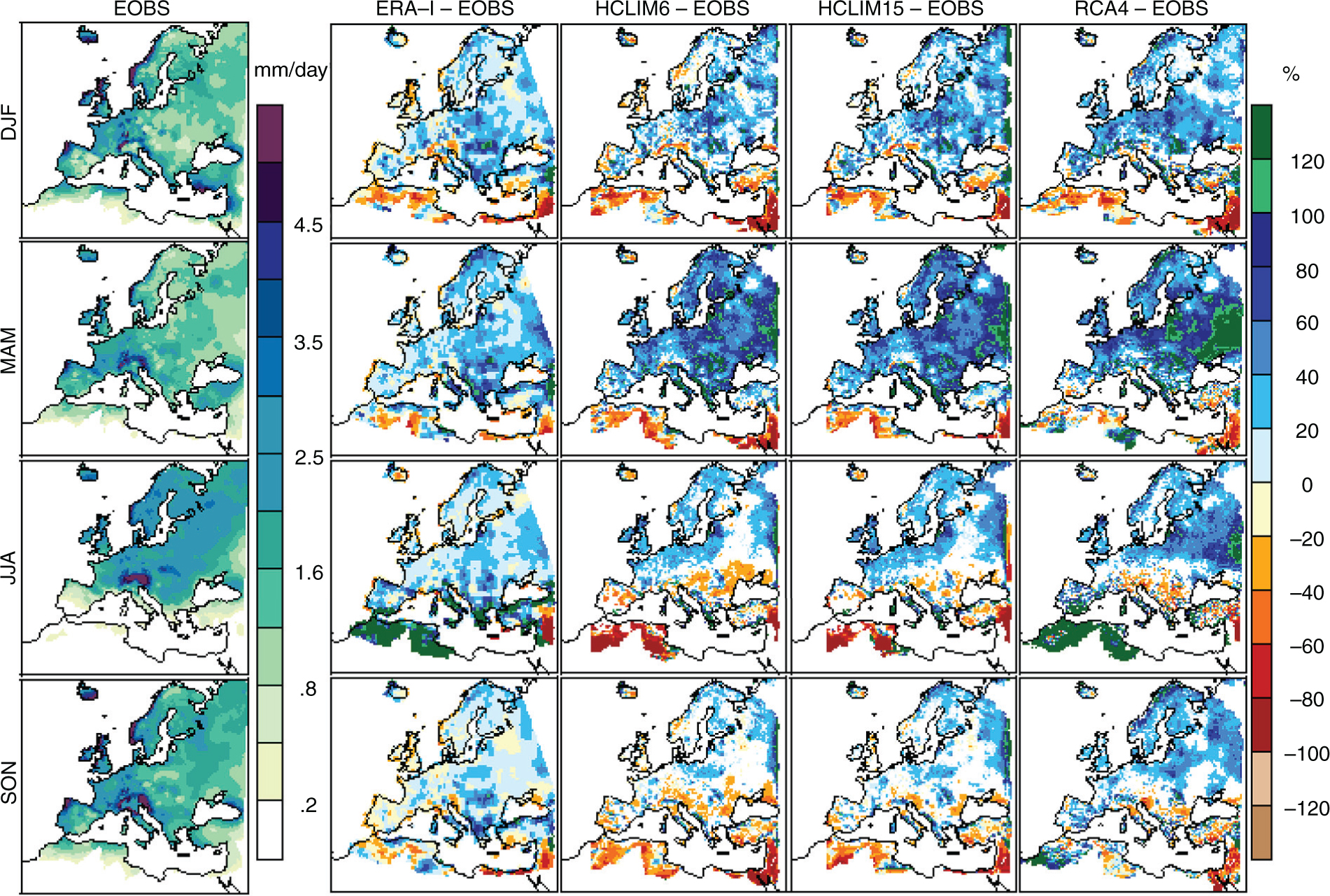
Fig. 7
Seasonal mean total precipitation. White areas (over land) indicate not statistically significant differences at the 5% level between model and observations and these grid points have been excluded. Absolute values of E-OBS and differences (%) with respect to ERA-I and RCMs.
Table 3. Statistics of seasonal precipitation for continental Europe
mean1.54±0.012.04±0.021.89±0.021.57±0.022.07±0.021.92±0.02nstd S
rmse S
R S 0.64±0.010.62±0.01
0.65±0.03
0.660.72±0.02
0.59±0.03
0.690.69±0.010.64±0.01
0.50±0.02
0.910.71±0.01
0.46±0.02
0.90nstd T
rmse T
R T 0.34±0.010.29±0.01
0.49±0.04
0.840.31±0.01
0.40±0.03
0.810.31±0.020.26±0.01
0.52±0.03
0.670.28±0.01
0.46±0.03
0.64
[i] Units are mm/day for mean and root mean square error (rmse). nstd is the normalised standard deviation and R is the coefficient of correlation. R and rmse are calculated between the HCLIM runs and E-OBS. Subscripts S and T refer to spatial and temporal, respectively. The uncertainty range is given by the 95% confidence interval from bootstrap computations using 1000 samples.
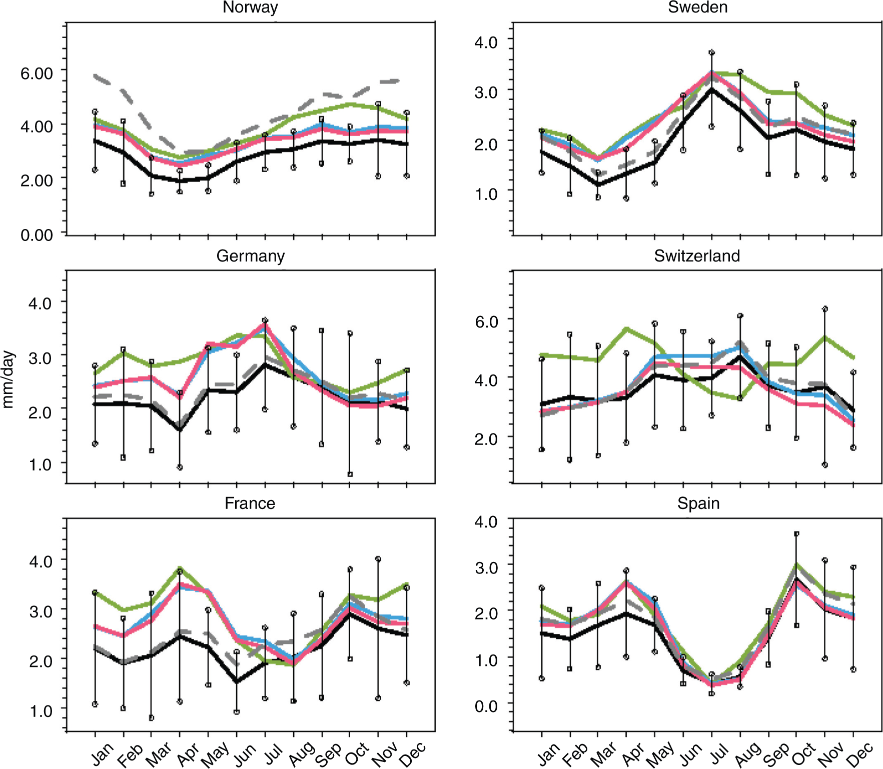
Fig. 8
Annual cycle of precipitation with reference to E-OBS (black), HCLIM6 (red), HCLIM15 (blue) and RCA (green). The vertical bars represent ±1 standard deviation based on the 10 yr of monthly values from E-OBS. The grey dashed lines are high-resolution observations (cf. Table 2)
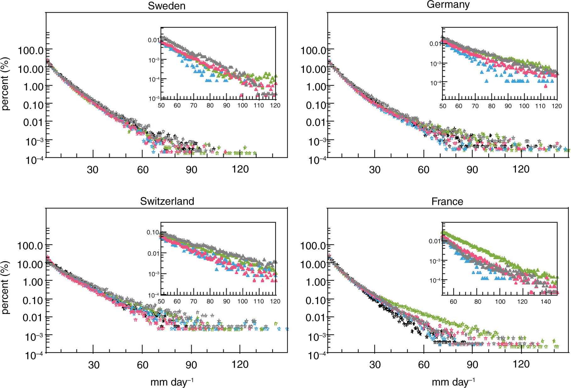
Fig. 9
The PDF of summer (JJA) daily mean precipitation in HCLIM6 (red), HCLIM15 (blue), RCA3 (green), E-OBS (black) and high-resolution observations (grey). Only wet days with a threshold of 1.0 mm/d are included. All data in main figures are aggregated to E-OBS grid. For the inset, model data are kept on native grid and observations are aggregated on to the HCLIM6 grid.
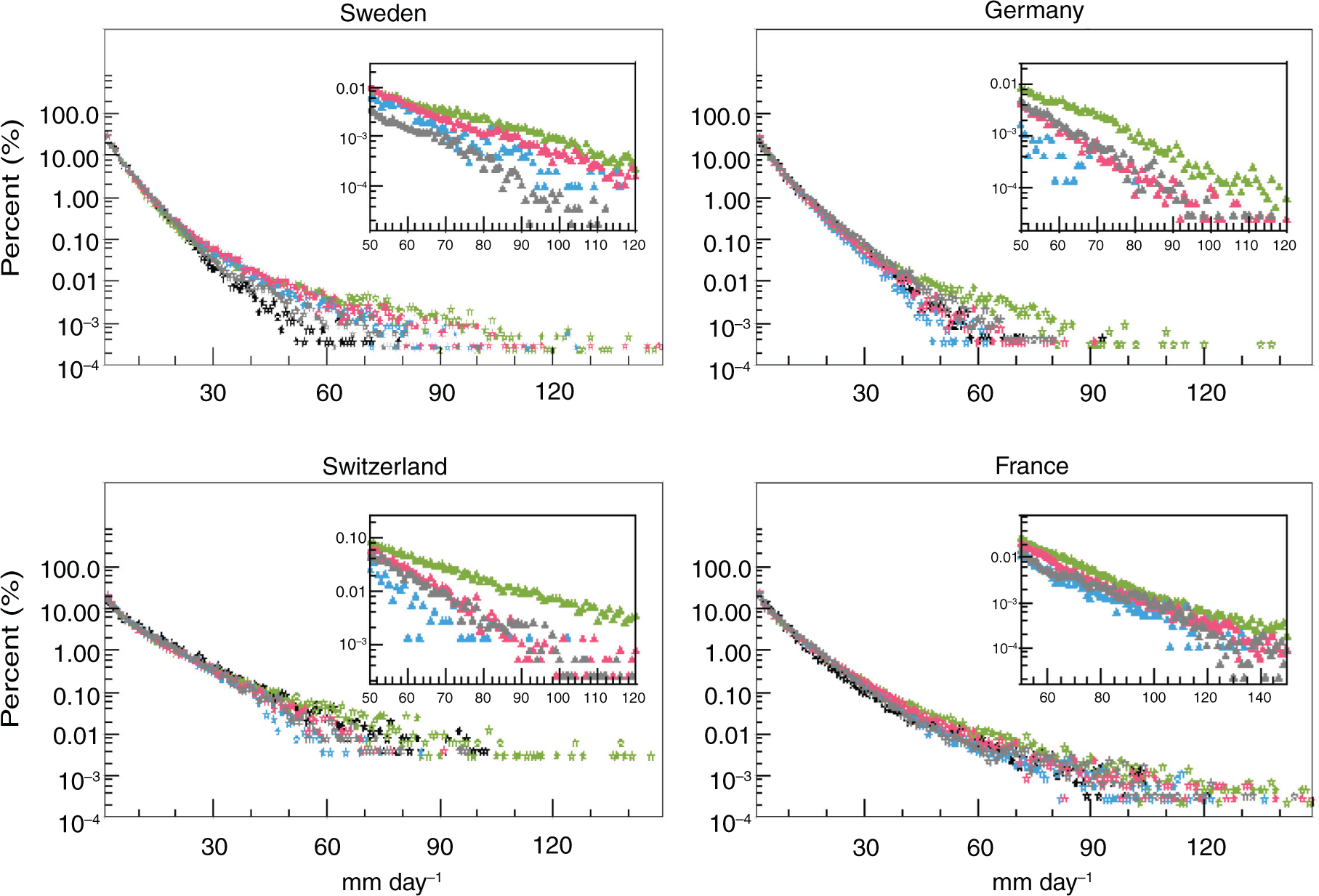
Fig. 10
The same as in Fig. 9 but for winter (DJF).
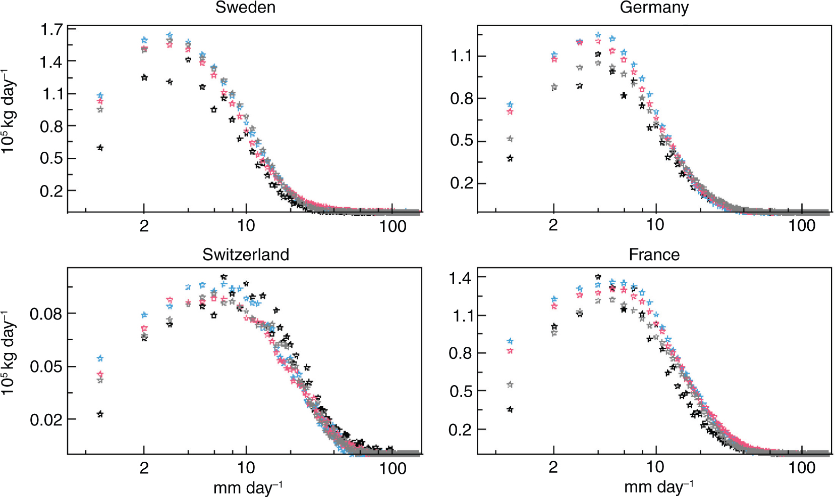
Fig. 11
Winter precipitation amount by rate. HCLIM6 (red), HCLIM15 (blue), E-OBS (black) and high-resolution observations (grey). See also Section 4.4.2.
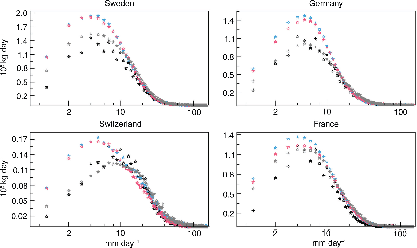
Fig. 12
Summer precipitation amount by rate, see Fig. 11.
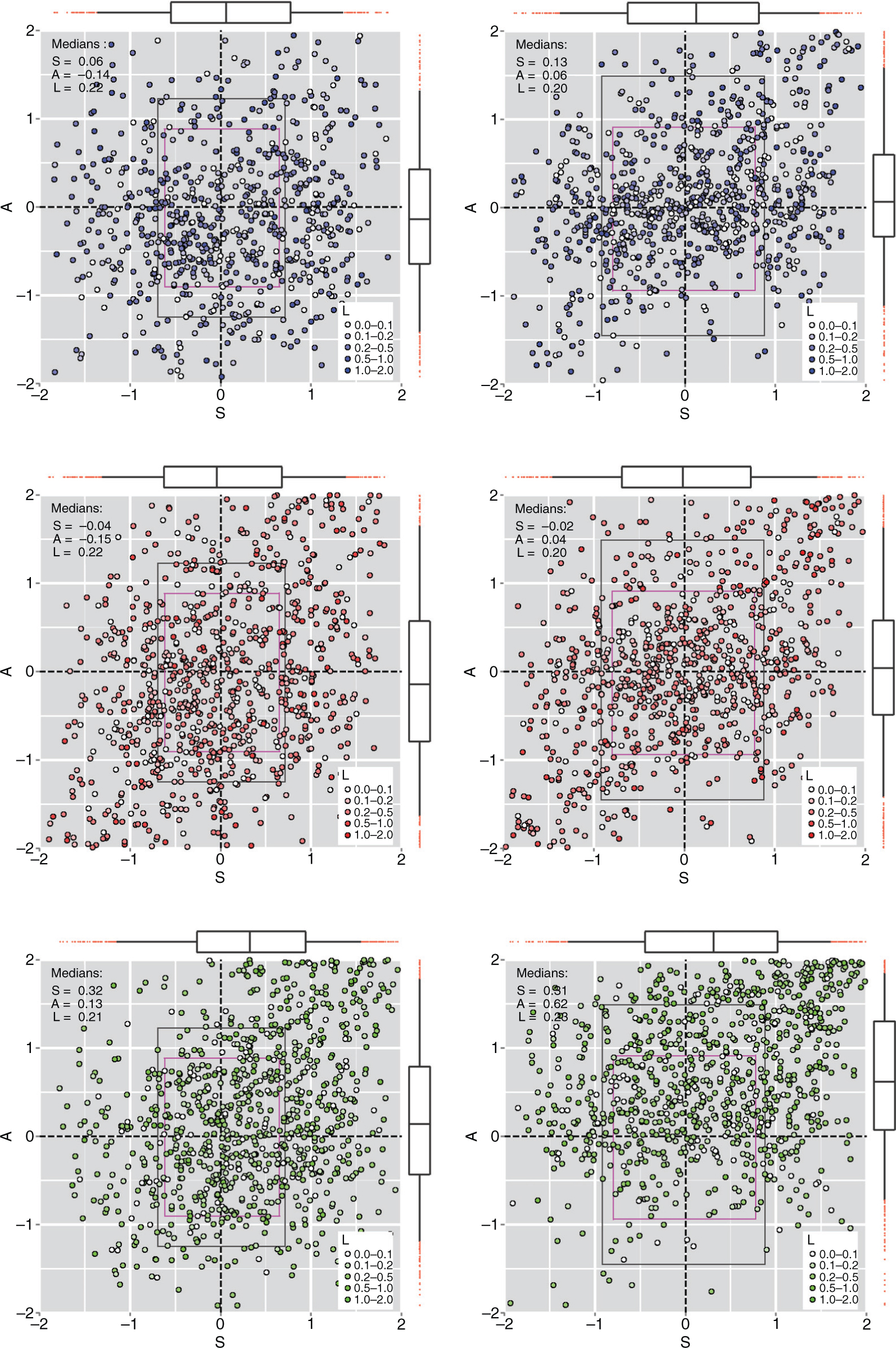
Fig. 13
Scatter plots of the SAL components structure (S, abscissa), amplitude (A, ordinate) and location (L, colour of dots) for two regions. The Alps (left column) and France (right) and for three simulations: HCLIM15 (top row), HCLIM6 (middle) and RCA3 (bottom). The box plots shows the distributions in S and A, representing 25th, 50th and 75th percentiles (the box), and the 5th and 95th percentiles (whisker). Grey and magenta rectangles illustrate the IQR of ‘random’ and ‘persistence’ forecasts, respectively.
Table 4. Median values of the three SAL components for four regions with the corresponding data set given in the parenthesis
SALSAL
HCLIM150.09 (1.58)0.29 (1.13)0.27 (0.26)0.06 (1.33)−0.14 (1.07)0.22 (0.20)HCLIM60.06 (1.62)0.37 (1.33)0.25 (0.22)−0.04 (1.30)−0.15 (1.36)0.20 (0.20)RCA30.32 (1.77)0.54 (1.17)0.29 (0.28)0.32 (1.20)0.13 (1.22)0.21 (0.21)France (SAFRAN)Norway (MetNo)
SALSALHCLIM150.13 (1.45)0.06 (0.93)0.20 (0.21)0.30 (1.38)−0.10 (0.88)0.33 (0.35)HCLIM6−0.02 (1.42)0.04 (1.07)0.20 (0.19)0.09 (1.23)−0.09 (0.94)0.31 (0.32)RCA30.31 (1.47)0.62 (1.23)0.23 (0.21)0.31 (1.36)−0.04 (1.05)0.37 (0.34)
Table 5. SAL space radius, r, calculated for the 5%, 10%, 20% and 50% points closest to a perfect score (i.e. to the origin)
5%10%20%50%5%10%20%50%
HCLIM150.400.540.761.220.390.490.681.07HCLIM60.420.550.731.240.390.520.691.16RCA30.420.580.761.360.370.490.671.08Persistence0.470.590.821.310.410.550.751.28Random0.530.690.991.590.500.680.931.55France (SAFRAN)Norway (MetNo)
5%10%20%50%5%10%20%50%HCLIM150.320.440.621.040.460.550.721.12HCLIM60.340.440.591.080.400.520.681.04RCA30.410.540.741.250.450.610.751.13Persistence0.500.630.851.370.400.490.651.08Random0.580.821.131.780.560.700.901.30