
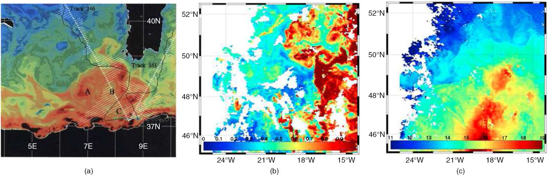
Fig. 1
Different examples of satellite images. (a) Altimetric reconstruction from JASON satellite data. (b) Ocean colour/Chlorophyll is from the MODIS captor of ENVISAT satellite. (c) Sea surface Temperature from the MODIS captor of ENVISAT satellite.
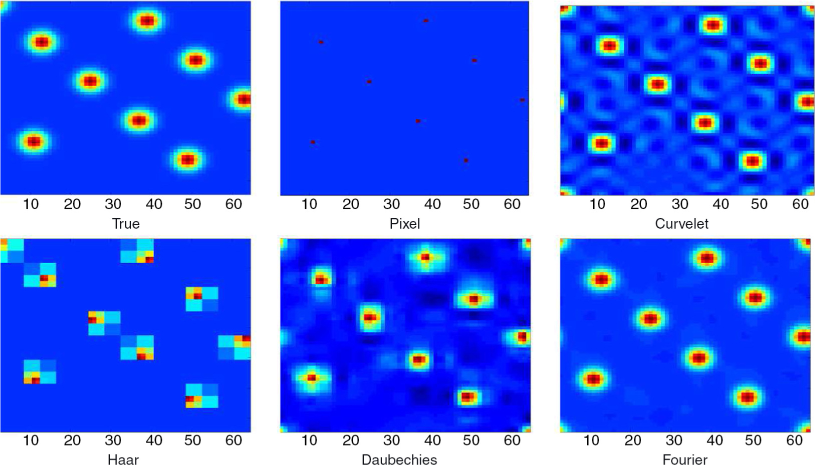
Fig. 2
Spatial correlations around nine selected points (top–left) and their representation with a diagonal approximation of the R matrix combined with various image transformations.
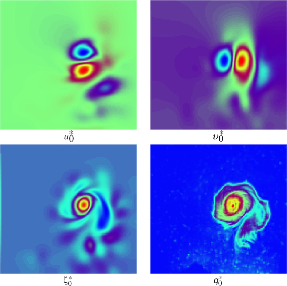
Fig. 3
Initial values of the scenario chosen for the twin experiments. The zonal and meridional velocities and are characterised by a strong vortex, illustrated by the initial vorticity . The height is assumed almost flat. The velocities take their values from −0.03 ms−1 (blue) to 0.04 ms−1 (red) and the 2-D vorticity from −0.2 s−1 (blue) to 0.64 s−1 (red). This synthetic initialisation has been created in order to match correctly the initialisation of the passive tracer, .
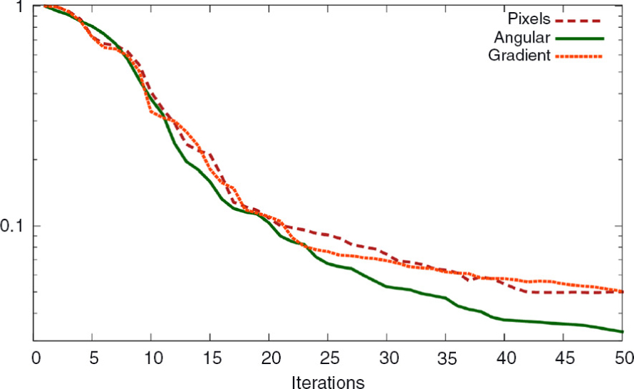
Fig. 4
Evolution of the ratio of RMS errors of the velocity u with respect to 4-D–Var iterations. Perfect data are observed and the three transformations are compared.
Table 1. Ratio between analysed state RMS and background state RMS for perfect data
Pixels4.7%3.5%11.4%24.5%Angular3.6%2.5%9.1%21.5%Gradient4.8%3.5%11.0%23.3%
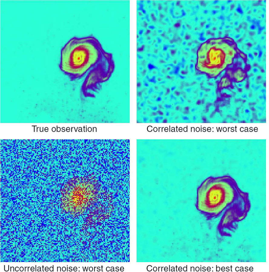
Fig. 5
First image of the sequence used for the assimilation, for various noise levels. The tracer concentrations vary from 0 (blue) to 1 (red). Top left: Perfect data scenario. Top right: Worst scenario tested for additive correlated Gaussian white noise (SNR=14.8 dB). Bottom left: Worst scenario for Gaussian white noise (SNR=6.7 dB). Bottom right: Best scenario for an additive correlated white noise (SNR=26.8 dB).
Table 2. Ratio between analysed state RMSE and background state RMSE, for the independent additive noise scenarios (Section 5.3)
Pix−Scalar61.7%32.0%11.1%5.3%∇−Block62.7%28.7%10.8%5.1%∇−ScalarDivergence48.8%12.3%4.7%Ang−Diag80.3%62.2%31.1%10.9%
Table 3. Ratio between analysed state RMSE and background state RMSE for data with spatially correlated additive noise of decreasing standard deviation
Pix−Scalar36.8%21.8%15.2%C−Diag8.3%7.7%8.1%Haar−Diag22.5%12.3%8.2%D8−Diag9.1%7.5%7.0%Fourier−Diag7.3%7.3%7.3%
Table 4. Ratio between analysed state RMSE and background state RMSE for data with spatially correlated additive noise of decreasing standard deviation
Pix−Scalar36.8%21.8%15.2%Pix−thinning(2)28.8%19.1%13.2%Pix−thinning(3)46.5%22.9%15.4%∇−Scalar20.2%13.5%11.1%Ang−Diag59.8%42.6%31.5%14.4%8.4%7.6%26.0%10.2%8.2%
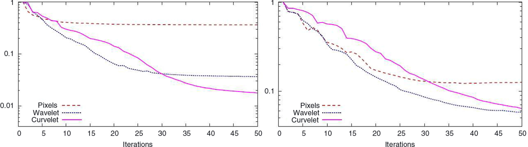
Fig. 6
Mean (over 10 experiments) cost function evolution with respect to 4-D–Var iterations (left). Mean (over 10 experiments) evolution of the RMSE ratio of v component of the velocity with respect to 4-D–Var iterations (right). Convergence rates are plotted for an isotropic noise. The noise magnitude is the smallest considered in the various experiments (26.8 dB).
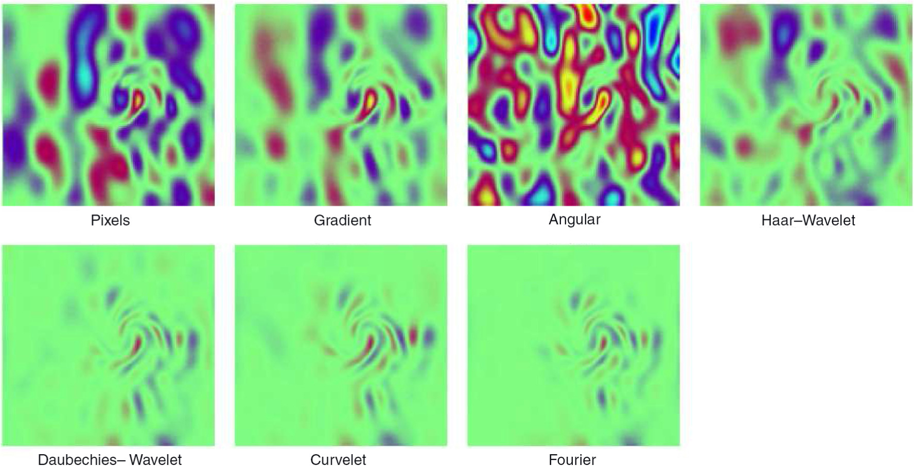
Fig. 7
Error analysis on the v–component of the velocity using the worst correlated image sequence studied. The velocity errors range from −0.0075 ms−1 (blue) to 0.0075 ms−1. The true velocity field (see Fig. 3) ranges from −0.025 ms−1 to 0.0405 ms−1.
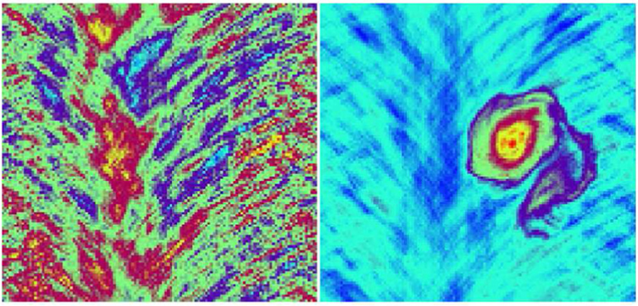
Fig. 8
Left: An example of anisotropic inhomogeneous Gaussian white noise. Right: A corrupted observation.
Table 5. Ratio between analysed state RMSE and background state RMSE for data with spatially correlated additive noise of decreasing standard deviation
Fourier−Diag23.5%13.8%8.2%C−Diag14.0%9.7%8.1%D8−Diag24.3%14.6%8.3%Pix–Scalar47.2%35.7%16.1%
[i] In this case an anisotropic and inhomogeneous noise (Section 5.5, see Fig. 8) is applied to the observations. The variable of interest is u.
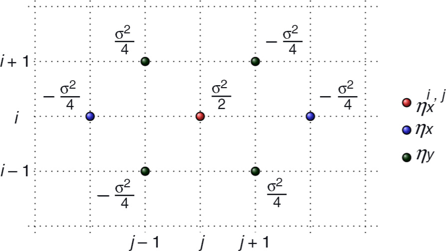
Fig. 9
Covariance between η x (i,j) (in red) and other elements (in green and blue) in a gradient space for an independent and identically distributed Gaussian white noise in the pixel space. The blue (resp. the green) points represents x– (resp. y–) derivative elements correlated to η x (i,j). All the covariances between η x (i,j) and other points are represented.
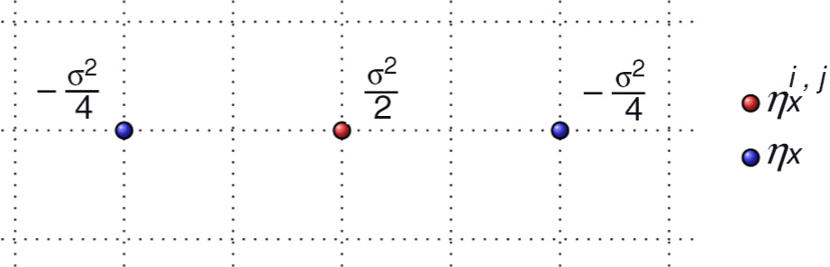
Fig. 10
Illustration of the simplification of the error covariance matrix. Only correlations between derivatives in the same direction are considered.