
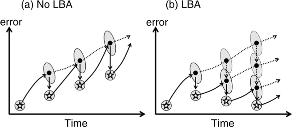
Fig. 1
Schematic of LBA. (a) without LBA and (b) with LBA. The x-axis represents the forecast time, and the y-axis is the forecast error. The stars and filled circles indicate analysis (initial conditions) and forecast (first guess), respectively. Solid arrows represent the forecast ensemble mean trajectory, and the dotted lines correspond to the LBC ensemble mean trajectory. Grey ellipses denote the ensemble spread for each analysis and forecast state.
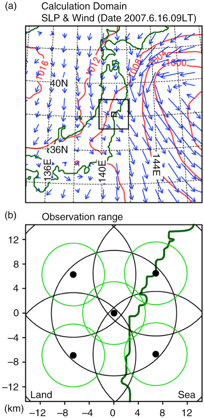
Fig. 2
(a) Calculation domain for the 12-, 2- and 0.4-km horizontal resolutions (solid squares), and surface weather map. Green lines correspond to the coastline. Red contours and arrows represent sea-level pressure and surface wind at 09:00 LT on 16 June 2007. (b) Lidar observation range at each site in the domain for the 0.4-km horizontal resolution. Black and green circles represent the observation range from each lidar for AS/ASLB and AS_h/ASLB_h, respectively. The Sendai airport is located at x=y=0.
Table 1. Outline of the experimental design for OSSE
TRUE0.4 km9:00 LT 16–9:00 LT 23 July 20071LBP2 km9:00 LT 16–9:00 LT 23 July 200721LETKF for initial conditions0.4 km14:15–18:00 LT 16 July 20072106:15–10:00 LT 17 July 200705:15–09:00 LT 19 July 2007LBA2 km14:15–18:00 LT 16 July 20072106:15–10:00 LT 17 July 200705:15–09:00 LT 19 July 2007Forecast cycle0.4 km14:00–18:00 LT 16 July 20072106:00–10:00 LT 17 July 200705:00–09:00 LT 19 July 2007 Each forecast starts with 15 minutes intervalExtended forecast experiments0.4 km14:00–18:00 LT 16 July 20072106:00–10:00 LT 17 July 200705:00–09:00 LT 19 July 2007Each 1-hour forecast starts with 15 minutes interval. See the detail in Section 4.2.
Table 2. List of experiments
NOASForecast without assimilationAS(AS1p)Analysis-forecast cycle without LBAASLB(ASLB1p)Analysis-forecast cycle with LBAAS2p, 4pSame as AS except with 2, or 4 lidar instrumentsASLB2p, 4pSame as ASLB except with 2, or 4 lidar instrumentsAS2p_h, 4p_hSame as AS2p, 4p except with half of lidar observation rangeASLB2p_h, 4p_hSame as ASLB2p, 4p except with half of lidar observation rangeF1h_AS1-hour forecast from the analysis of ASF1h_ASLB1-hour forecast from the analysis of ASLB
Table 3. Outline of case studies
Duration14:00–18:00 LT 16 July 200706:00–10:00 LT 17 July 200705:00–09:00 LT 19 July 2007Representation of TRUEWesterly more than 10 m s−1, clear sea-breeze front.Calm condition (<2 m s−1), sea-breeze is 400 m thickness.Northwesterly of 5–7 m s−1, sea-breeze is 200 m thickness.
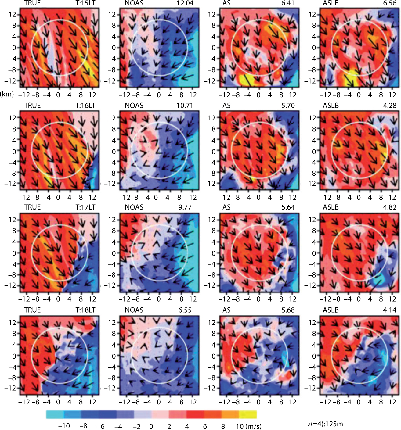
Fig. 3
Horizontal wind (arrows) and the structure of east–west wind speed (shades) at 125-m height. From the left panels, TRUE, NOAS, AS and ASLB are displayed with 1-hour interval. Panels of AS and ASLB are analysis ensemble mean. Numbers on the upper right corner of each panel indicate UTC for TRUE and area-averaged RMSEs for NOAS, AS and ASLB. Circle in each figure denote the observation range. The x- and y-axes are the distance from the centre of calculation domain.
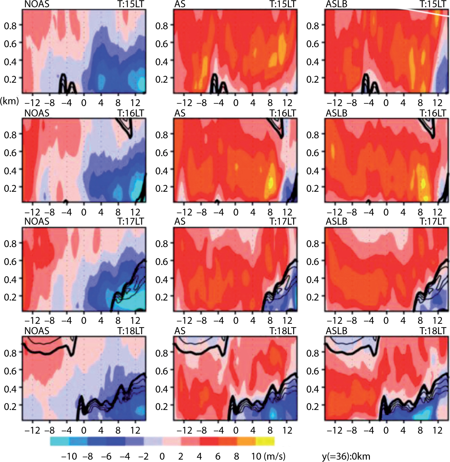
Fig. 4
Sea-breeze vertical structures with time interval of 1 hour in the NOAS, AS and ASLB. Panels of AS and ASLB are analysis ensemble mean. Shades indicate east–west wind speed at y=0 km. Contours denote east–west wind speed with the values of −6, −4, −2, 0 m s−1 in the TRUE. Thick contours indicate the boundary between sea-breeze and westerly.
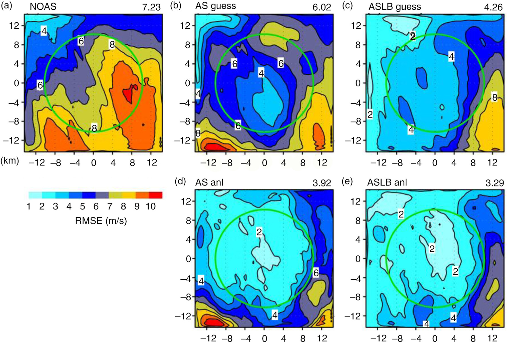
Fig. 5
Vertically averaged RMSE of wind speed, from surface to 1-km height in the NOAS, AS and ASLB. For the AS and the ASLB, first guess and analysis are displayed. Circle in each figure denote the observation range.
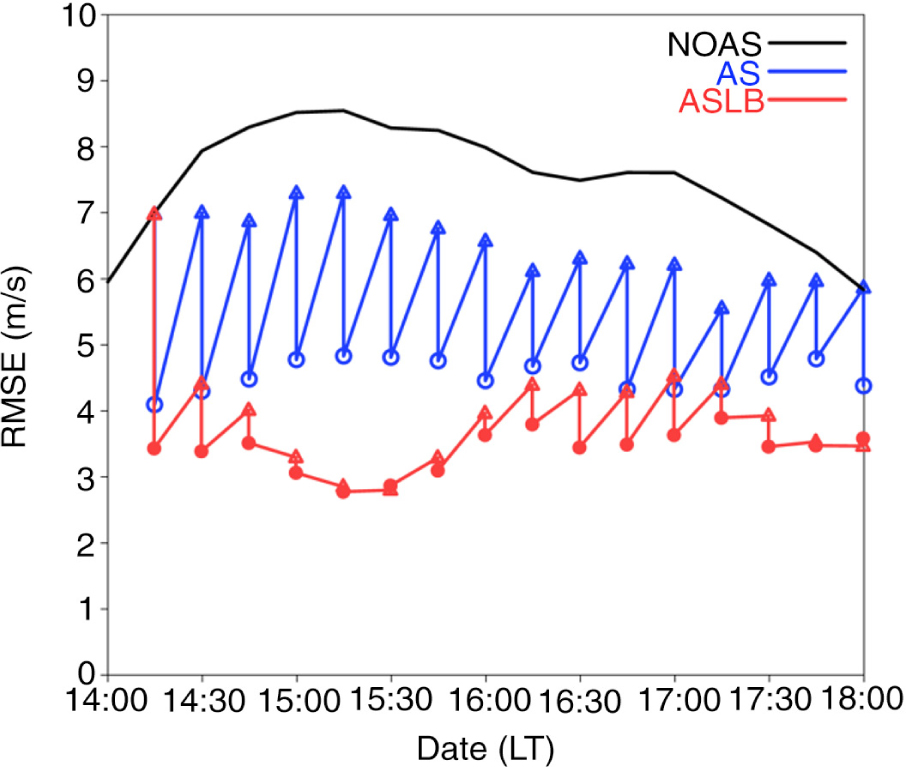
Fig. 6
Domain-averaged RMSE of wind speed from surface to 1-km height for the analysis–forecast cycle in the NOAS (black), AS (blue) and ASLB (red). The x-axis denotes the forecast date and the y-axis is the averaged RMSE. Circles and triangles represent analysis and first guess.
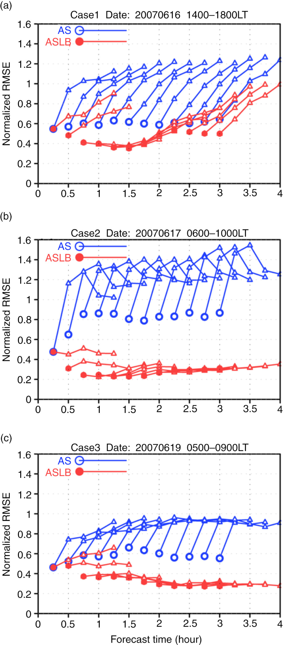
Fig. 7
Domain-averaged normalised RMSEs by the RMSE of NOAS at each forecast which have different initial times in the three cases. Circles and triangles represent analysis and first guess. Blue and red lines indicate F1h_AS and F1h_ASLB experiments.
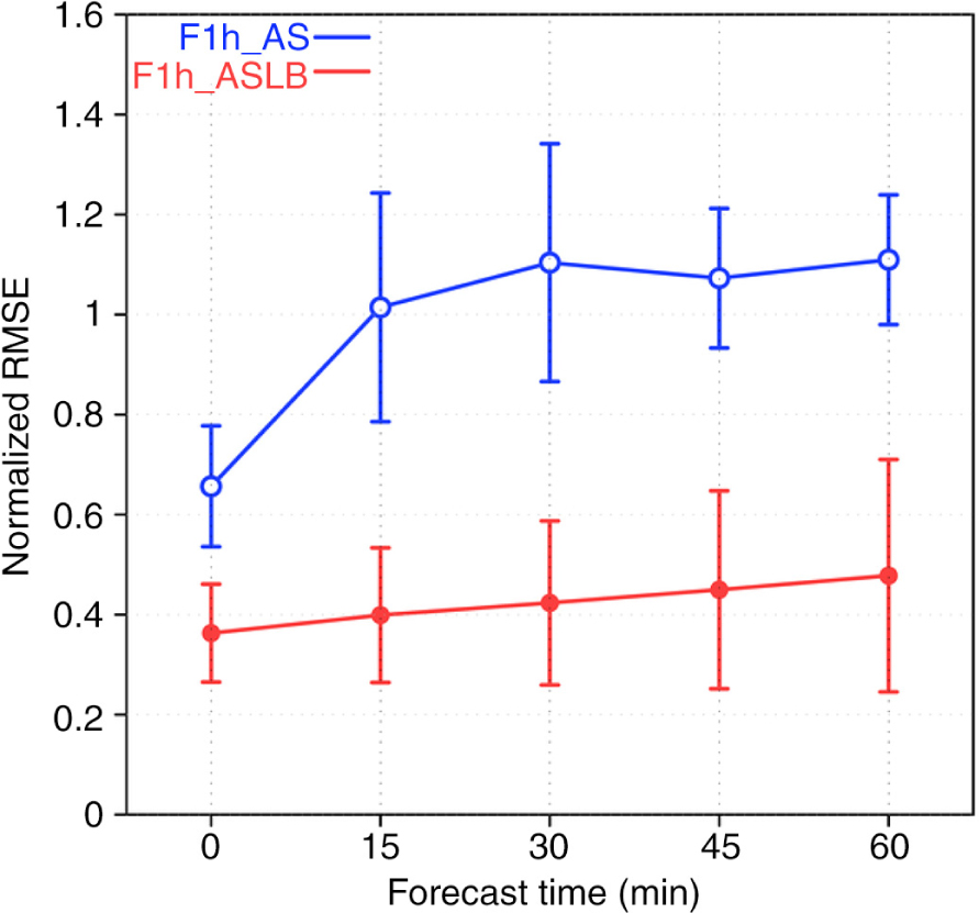
Fig. 8
The ensemble averaged normalised error growth by the NOAS. Blue and red lines indicate F1h_AS and F1h_ASLB experiments. Bars over the circles indicate one standard deviation. The x-axis corresponds to the forecast length from analysis.
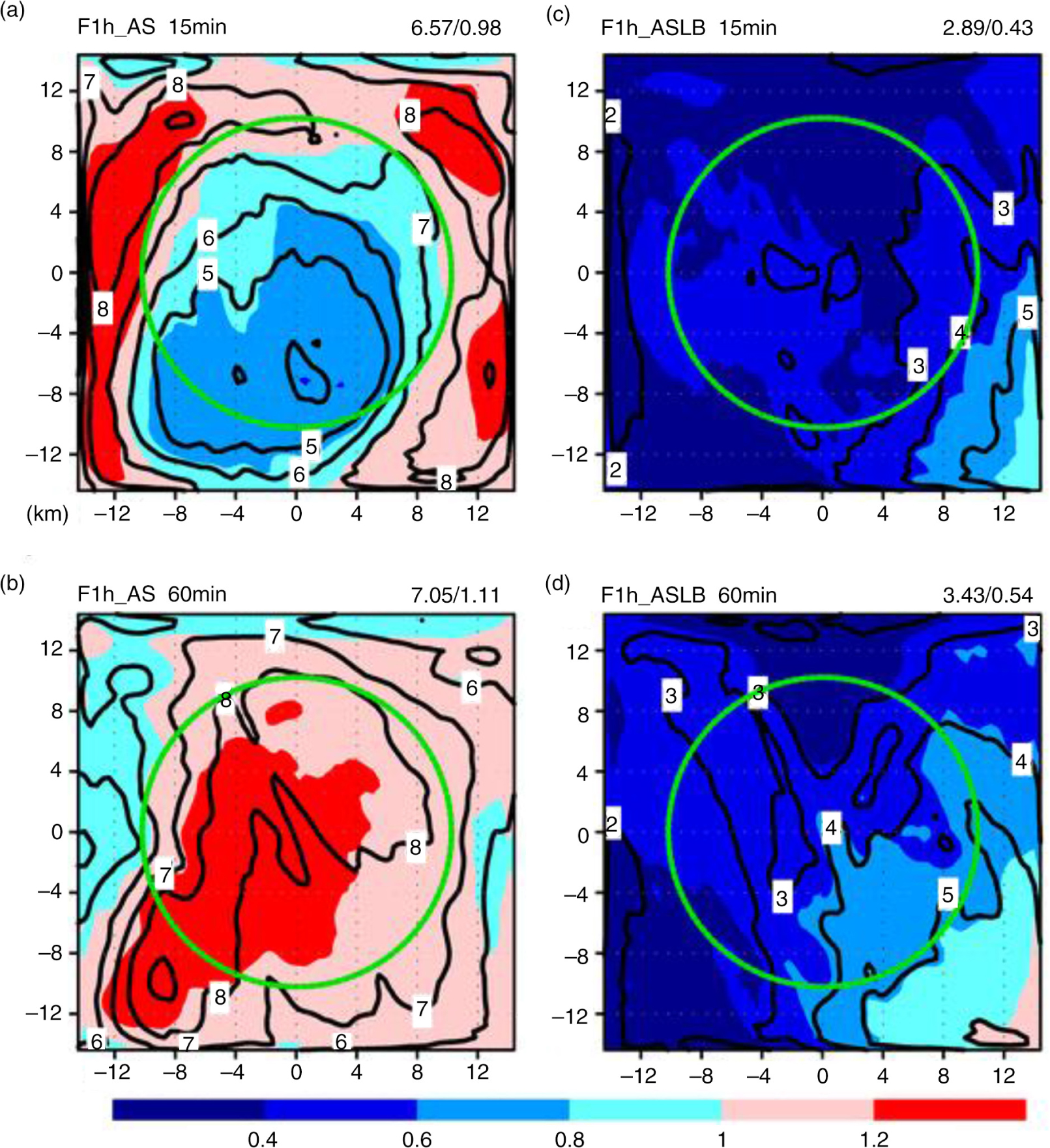
Fig. 9
Horizontal distribution of the normalised RMSE by the RMSE of NOAS in the (a), (b) F1h_AS, and (c), (d) F1h_ASLB. Upper panels refer to the 15 minutes forecast and the lower panels to the 60 minutes forecast. Contours and shades indicate the RMSE with the interval of 1 m s−1 and the normalised RMSE. These are averaged for 36 cases. Numbers on the upper right corner of each panel are the domain-averaged RMSE and normalised RMSE. Circle in each figure denote the observation range.
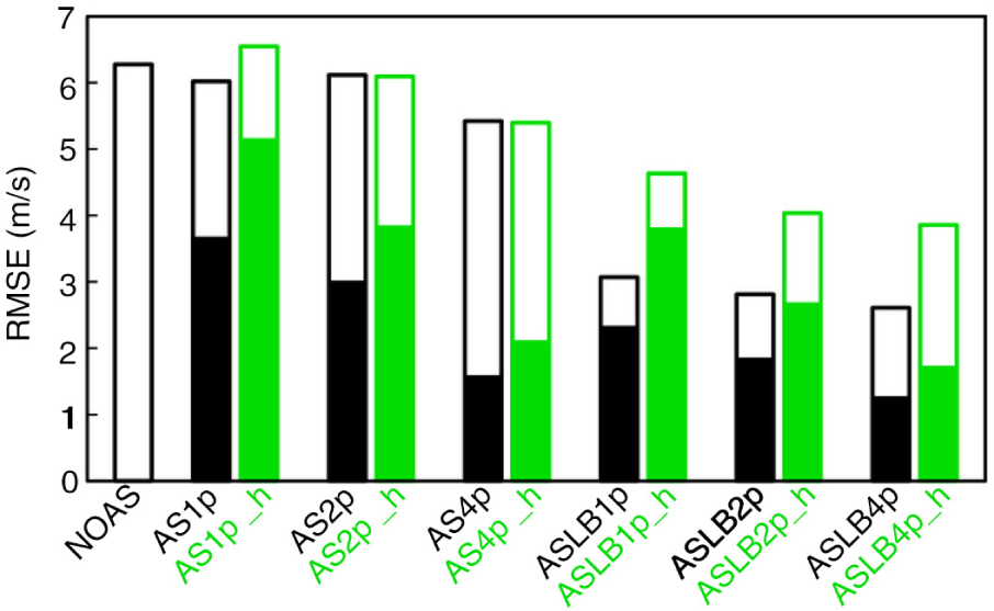
Fig. 10
The domain-averaged RMSEs of wind speed in the NOAS, AS1p, AS2p, AS4p, ASLB1p, ASLB2p, ASLB4p, AS1p_h, AS2p_h, AS4p_h, ASLB1p_h, ASLB2p_h and ASLB4p_h. Filled and open bars indicate analysis and first guess (15-minute forecast) errors, respectively. The y-axis is RMSE (unit is m s−1).