
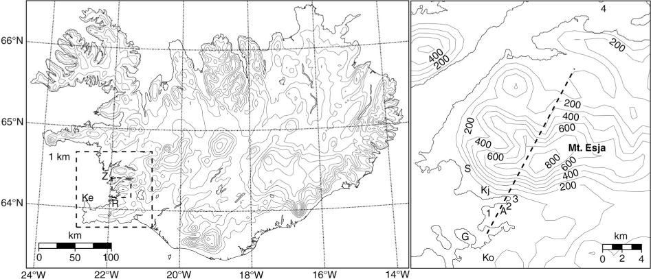
Fig. 1
Model topography (left, 200 m contours) at 3 km resolution, and in the main region of interest (Z) within the 1-km resolution domain (right, 100 m contours). The locations of RPAS flights (1, 2 and 3), the pseudo temperature sounding used in the sensitivity test (4), a section across Mt. Esja (dashed line), and stations at Keflavík (Ke), Reykjavík (R), Geldinganes (G), Korpa (Ko), Álfsnes (A), Kjalarnes (Kj) and Skrauthólar (S) are shown.
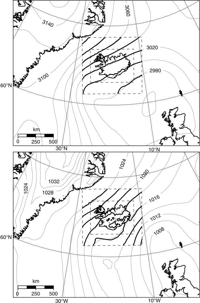
Fig. 2
Geopotential height at 700 hPa [m] (above) and mean sea level pressure [hPa] (below) at 1200 UTC on 15 July 2009 (ECMWF Interim re-analysis). Also shown are the same fields simulated (NO) at 9 km horizontal resolution (bold), as well as the 9 and 3 km domain limits (dashed lines).
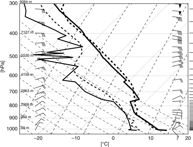
Fig. 3
Skew-T diagram from the Keflavík upper-air station in Southwest-Iceland at 1200 UTC on 15 July 2009 (cf. Fig. 1 for location). Shown are observed (solid lines) and simulated (NO) at 1 km resolution (dashed lines) temperature and dew point [°C] as well as wind barbs (2.5 ms−1 each half barb, observed to the right and simulated to the left) with temperature/dew point on the lower axis and height [hPa] on the vertical. Also indicated are the heights of some of the pressure levels as well as the height of model levels (extreme right).
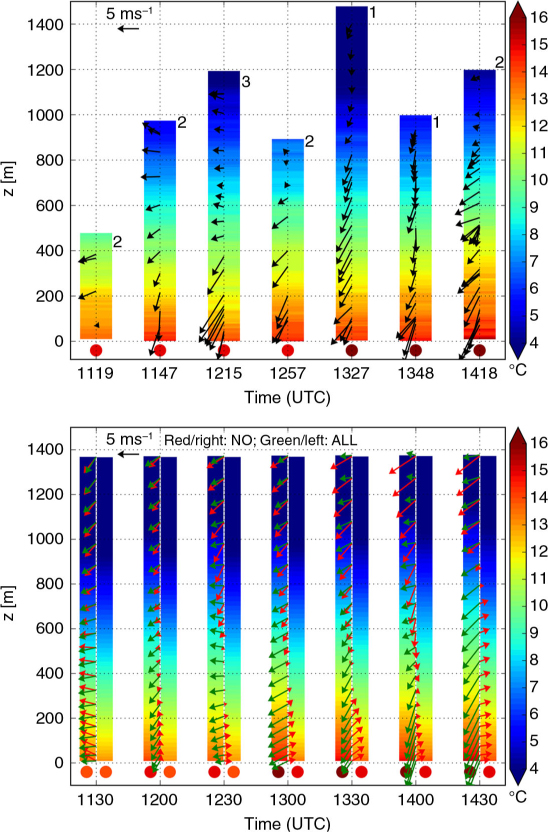
Fig. 4
Observed and simulated vertical profiles of winds [ms−1] and temperature [°C] (bars), as well as 2-m temperature (dots) on 15 July 2009. Observed profiles (above) are from the descending part of the RPAS flights (locations indicated at top of bars and in Fig. 1), with 2-m temperature from Álfsnes. Simulated surface temperature and profiles (below) are from the NO (red arrows/right column) and ALL (green arrows/left column) 1 km domains and they are taken at/above the Álfsnes automatic weather station (Fig. 1).
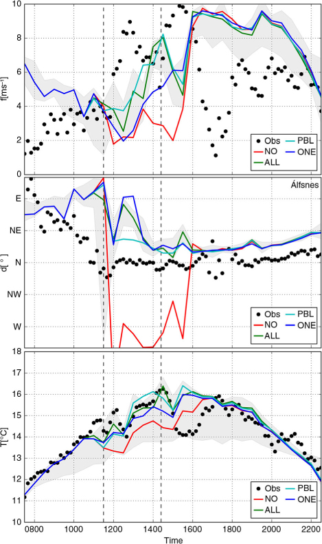
Fig. 5
Observations and simulations (1 km resolution) of 10-m surface wind speed [ms−1] (above) and direction [°] (centre), as well as 2-m temperature [°C] (below) at Álfsnes (location A in Fig. 1). The spread of the simulated values (ALL) in a 3×3 km2 area centred on the station location is bounded within the grey envelope. The dashed, vertical, lines indicate the time interval with available RPAS observations.
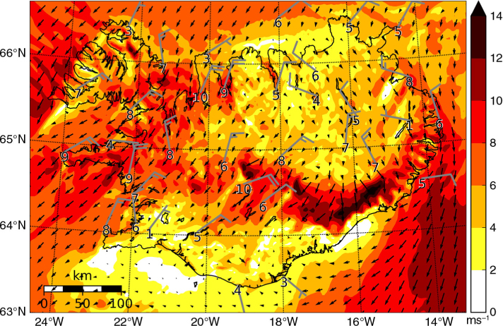
Fig. 6
Simulated 10-m wind speed [ms−1] and wind vectors at a horizontal resolution of 3 km (NO), as well as observed 10-m winds at automatic weather stations (numbers and barbs, 2.5 ms−1 each half barb), at 1200 UTC on 15 July 2009.
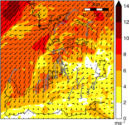
Fig. 7
Simulated 10-m wind speed [ms−1] and wind vectors at a horizontal resolution of 1 km (NO), as well as observed 10-m winds at automatic weather stations (numbers and barbs, 2.5 ms−1 each half barb), at 1200 UTC on 15 July 2009.
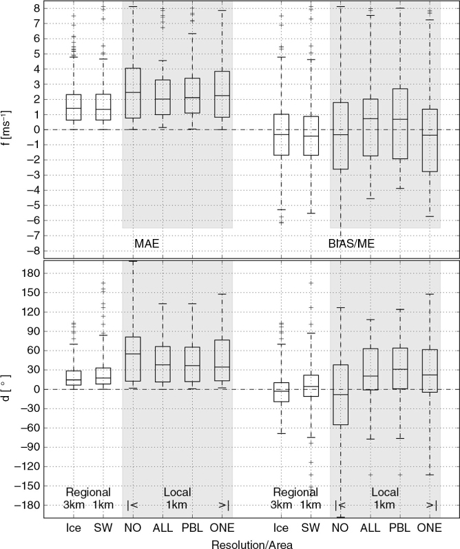
Fig. 8
Mean absolute error (MAE) and mean error (BIAS/ME) for simulated wind speed (above) and direction (below). The regional flow in Iceland (Ice, 3 km) and Southwest-Iceland (SW, 1 km) is presented based on the NO simulation. The local flow in the main region of interest is presented for five stations (Fig. 1; S, Kj, A, G and Ko) and the NO, ALL, PBL and ONE 1 km simulations (shaded region). The median is given by the horizontal line inside the box which covers the 25% and 75% quartiles, while whiskers show the range of the data, excluding outliers.
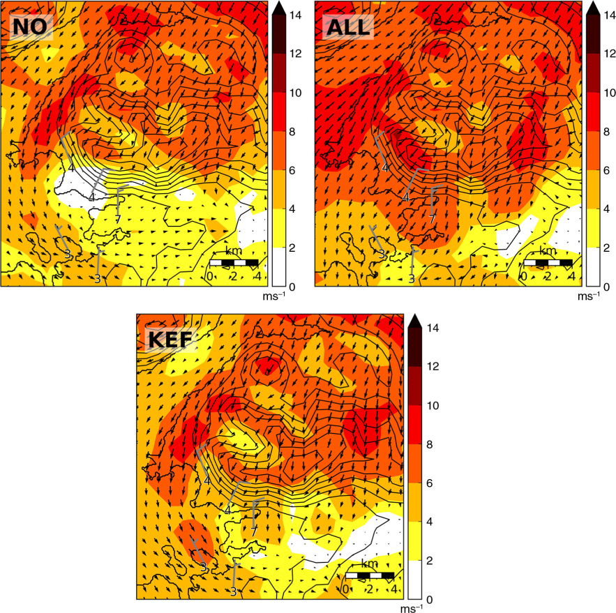
Fig. 9
Simulated 10-m wind speed [ms−1] and wind vectors at a horizontal resolution of 1 km in the NO (upper left), ALL (right) and KEF (below) simulations, as well as observed 10-m winds at automatic weather stations (numbers and barbs, 2.5 ms−1 each half barb), at 1400 UTC on 15 July 2009. Terrain contours with 100 m interval.
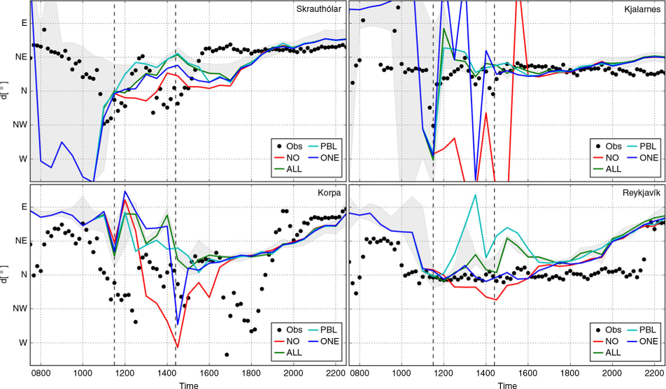
Fig. 10
Observed and simulated 10-m wind direction [°] at four automatic weather stations on 15 July 2009. Simulated values are from the 1 km horizontal domain for the control run (NO) and three nudged runs. The spread of the simulated values (ALL) in a 3×3 km2 area centred on the station location is bounded within the grey envelope. The dashed, vertical, lines indicate the time interval with available RPAS observations.
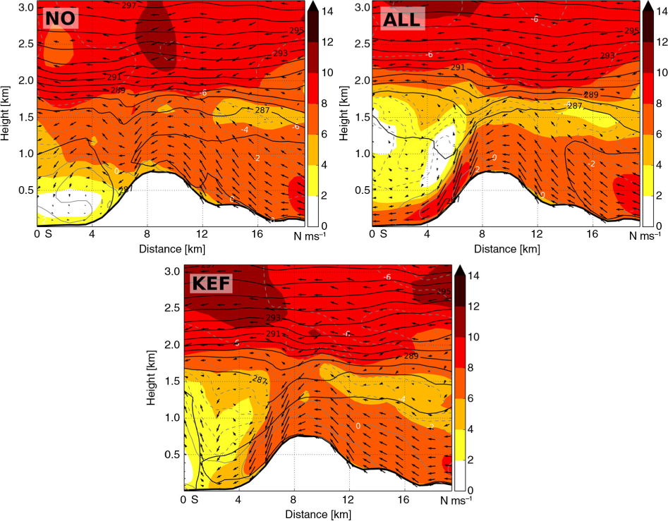
Fig. 11
Wind speed [ms−1], wind vectors in the plane (vertical wind scaled by 10) and isentropes [K] at 1 km resolution in the NO (upper left), ALL (right) and KEF (below) simulations in a section across Mt. Esja, at 1400 UTC on 15 July 2009. Also shown is orography, as well as grey lines indicating, respectively, flow out of (solid) and into (dashed) the section with a 1ms−1 interval.
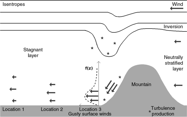
Fig. 12
A schematic summary depicting the presumed gravity wave activity aloft and the lee-side accelerated flow, as well as observed wind profiles in lee of the mountain.