
Fig. 1
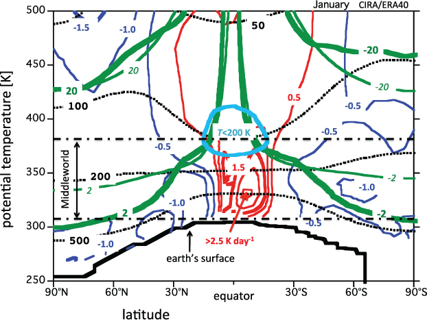
January average zonal mean pressure (dotted black lines, labelled in units of hPa), potential vorticity (thick green lines, labelled in PVU), reference potential vorticity (thin green lines, labelled in PVU), cross-isentropic flow (labelled in units of K day−1; blue: downwelling; red: upwelling) and temperature (cyan; only the 200 K isotherm) as a function of latitude and potential temperature, according to the ERA-40 re-analysis (Uppala et al., 2005) and CIRA (Fleming et al., 1990). The thick black line indicates the zonal mean position of the earth’ surface. The black dashed–dotted lines indicate the top and bottom of the Middleworld. The ERA-40 average is for the period 1979–2002. ERA-40 data: provided by Paul Berrisford.
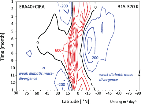
Fig. 2
Average yearly cycle of the diabatic convergence of mass per unit area into the Middleworld layer between θ=315 K and θ=370 K. Labels indicate diabatic mass flux convergence in units of kg m−2 day−1. The figure is based on the ECMWF ERA-40 re-analysis of the monthly mean zonal mean diabatic heating and the monthly mean isentropic density at θ=315 K and at θ=370 K, according to the CIRA (Fleming et al., 1990).
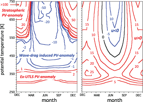
Fig. 3
Left panel: yearly cycle of the area-weighted amplitude of the monthly mean PV-anomaly north of 65°N, as a function of time and potential temperature. Red contours: positive anomaly; blue contours: negative anomaly. Labels are in units of PVU. The ±1, ±2, ±5, ±10, ±20, ±50 and ±100 PVU contours are drawn. Right panel: yearly cycle of the area-weighted zonal wind between 30°N and 60°N. Contour interval is 5 m s−1. Labels are indicated in units of m s−1. Based on the CIRA (Fleming et al., 1990).
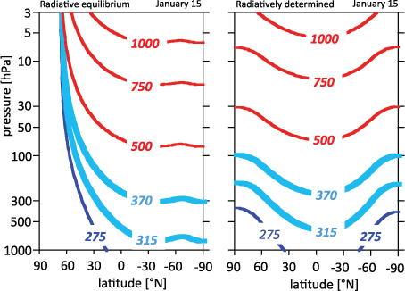
Fig. 4
Radiative equilibrium potential temperature (left panel) and radiative determined potential temperature (right panel), labelled in K, as a function of latitude and pressure on 15 January for an atmosphere which is transparent to solar radiation and contains one well-mixed greenhouse gas. The albedo of the earth's surface is 0.3. The result shown in the right panel is for C=5×10⁷ J K−1 m−2. The cyan contours represent isentropes in the Middleworld. The red contours represent isentropes in the Overworld. The dark blue contour is an isentrope in the Underworld. In the Polar night poleward of about 67°N, the radiative equilibrium temperature is absolute zero Kelvin (left panel).
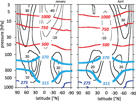
Fig. 5
Observed (CIRA: COSPAR International Reference Atmosphere) monthly average zonal average potential temperature, labelled in K (blue: Underworld; cyan: Middleworld; red: Overworld), and zonal mean zonal wind (black), labelled in m s−1, as a function of latitude and pressure for January (left panel) and for April (right panel).
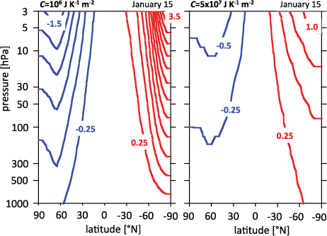
Fig. 6
‘Radiatively determined’ cross-isentropic flow (labelled in units of K day−1; contour interval is 0.25 K day−1; zero contour not drawn) as a function of latitude and pressure for January 15 (in the fourth year), for two values of the thermal inertia coefficient, C: in the left panel C=106 J K−1 m−2; in the right panel C=5×10⁷ J K−1 m−2. The atmosphere is assumed to be transparent to solar radiation and contains one well-mixed greenhouse gas. The earth's surface albedo is 0.3 [see the text below eq. (13)].
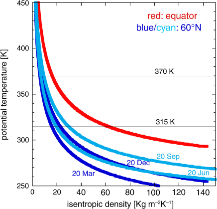
Fig. 7
‘Radiatively determined’ isentropic density, σ rad, as function of potential temperature at the equator and at 60°N, for four different ordinal dates in year 3 of the integration of the radiation model for an atmosphere containing one well mixed greenhouse gas (see the text) and with C=5×10⁷ J K−1 m−2. The ordinal dates are 20 March, 20 June, 20 September and 20 December. The isentropic density profile at the equator is nearly identical for all four dates. The layer between 315 K and 370 K represents the Middleworld, which lies in the tropical troposphere and in the extratropical stratosphere.
Table 1. Absorption cross-sections of ozone (per molecule) and of water vapour (per kg) in the four solar spectral bands
112×10−22026.52×10−2403422×10−250450.500.002
Table 2. Overview of the physics that is included (‘yes’) or excluded (‘no’) in 15 model runs, along with the values of obliquity, δ max, thermal inertia coefficient, C [eq. (15)], and the latitude of maximum advance toward the pole of the ITCZ, φ max
1a0.05×107NoNoNoNo–51b0.0106NoNoNoNo–51c0.05×107NoNoYesNo–51d0.05×107NoNoNoYes0.061e0.05×107NoNoYesYes0.061f0.05×107NoYesYesYes0.06/72a23.455×107NoNoNoNo–82b23.455×107YesNoNoNo–82c23.455×107YesNoYesNo–83a23.455×107YesYesNoYes23.4583b23.455×107YesYesYesYes23.4583c23.455×107YesNoYesNo–83d23.45107YesYesYesYes23.4584a23.455×107YesYesYesYes10.084b23.45106YesYesYesYes10.08
[i] The last column indicates the section in which the run is discussed. Each run is initialised on January 1 with an isothermal atmosphere (290 K) at rest. The total length of each run is 4 yr. Solar radiation (SR) is absorbed by ozone (if present), water vapour (if present) and the earth's surface. The ozone concentration is prescribed according to the analysis of observed zonal mean, monthly mean values due to Fortuin and Kelder (1998). The water cycle is described in section 6. The wave drag coefficient, D 0 [eq. (25)] is –5×10⁻⁵ m s−2 in all experiments. Furthermore, z 0=10 km and z 1=25 km. Animations of selected runs can be viewed in the supplementary files.
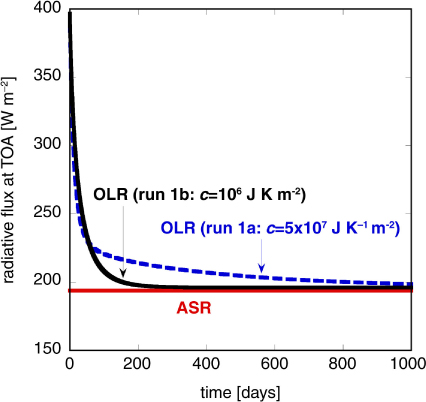
Fig. 8
Global average absorbed solar radiation at the top of the atmosphere and global average outgoing long wave radiation at the top of the atmosphere in runs 1a and 1b, which differ only in the value of the thermal inertia coefficient, C.

Fig. 9
Permanent equinox equilibrium state without (run 1a, left panel) and with (run 1c, right panel) wave drag, in an atmosphere lacking water (Table 2). Isentropes are labelled in units of K (blue: Underworld; cyan: Middleworld; red: Overworld), zonal wind (u) (black; labelled in units of m s−1; contour interval is 5 m s−1), wave drag, D [eq. (25)] (the dotted line corresponds to D= − 2.5×10⁻⁵ m s−2) and the dynamical tropopause (green line, labelled in PVU), as a function of latitude and pressure. Due to symmetry around the equator, only the northern hemisphere is shown.
Table 3. The values and units of model parameters associated with the water cycle
σ m 0.3m2 kg−1σ v 0.125m2 kg−1RH g 75%rITCZ1500kmFlp0.8Dimensionlessp cb 900hPap ct0 400hPaΔp ct −200hPaH v 2100mB0.3Dimensionless
[i] The parameters σ m and σ v are the long-wave absorption cross-sections of the well-mixed greenhouse gas and water vapour, respectively. Support for the parameter values, which are related to cloud base and cloud top, is given in the paper by Schumacher et al. (2004).

Fig. 10
Zonal mean precipitation, averaged for the years 1979–2012, according to the ERA-Interim re-analysis (Dee et al., 2011), as a function of latitude (solid line), and the equilibrium precipitation in run 1f (dashed line).
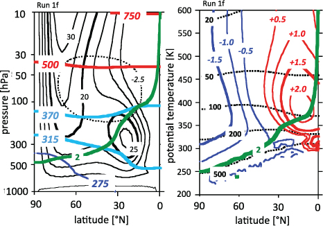
Fig. 11
Permanent equinox equilibrium state in run 1f, including wave drag and the water cycle (Table 2). Left panel: potential temperature, zonal wind and wave drag as a function of latitude and pressure. Isentropes are labelled in units of K (blue: Underworld; cyan: Middleworld; red: Overworld), zonal wind (u) (black lines, labelled in units of m s−1; contour interval is 5 m s−1), wave drag, D [eq. (25)] (the dotted line corresponds to D=− 2.5×10⁻⁵ m s−2) and the dynamical tropopause, shown in green (labelled in PVU). Right panel: cross-isentropic flow (labelled in units of K day−1; blue: downwelling; red: upwelling) and pressure (dotted lines labelled in units of hPa) as a function of latitude and potential temperature. Due to symmetry around the equator, only the northern hemisphere is shown. Animations of run 1f can be viewed in the supplementary file.
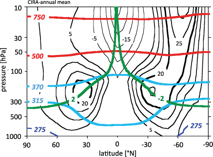
Fig. 12
The CIRA-annual mean state in terms of potential temperature, labelled in K (blue: Underworld; cyan: Middleworld; red: Overworld), and zonal mean zonal wind (black contours, labelled in m/s) as a function of latitude and pressure. The green contour represents the dynamical tropopause (labelled in PVU).
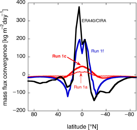
Fig. 13
Steady state diabatic mass flux convergence per unit horizontal area into the Middleworld layer between θ=315 K and θ=370 K as a function of latitude, in the permanent equinox runs 1a, 1c and 1f (Table 2), as well as an estimate of the annual mean of this quantity in reality, based on the ERA-40 re-analysis (Fig. 2).
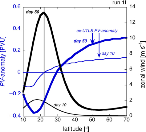
Fig. 14
Latitude dependence at θ=350 K of the zonal wind (black) and of the PV-anomaly, Z′, [eq. (5)] (blue) on day 10 and day 50 of run 1f (Table 2).
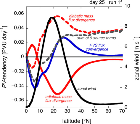
Fig. 15
Latitude dependence at θ=350 K of the zonal wind (solid black) and of the first three PV-source terms on the r.h.s. of eq. (40) on day 25 of the permanent equinox run 1f (Table 2). The grey dashed line represents the sum of all five terms on the r.h.s. of eq. (40).

Fig. 16
As in Figure 3, but for year 3 of run 3b. Labels in left panel are in units of PVU. Labels in right panel are in are in units of m s−1.
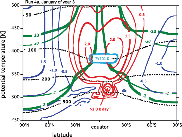
Fig. 17
January average in year 3 of run 4a (Table 2) of zonal mean pressure (dotted black lines, labelled in units of hPa), potential vorticity (thick green lines, labelled in PVU), reference potential vorticity (thin green lines, labelled in PVU), cross-isentropic flow (labelled in units of K day−1; blue: downwelling; red: upwelling) and temperature (cyan; only the 201 K isotherm) as a function of latitude and potential temperature. An animation of run 4a can be viewed in the supplementary file.

Fig. 18
Annual mean state in year 3 in run 4a (Table 2) in terms of potential temperature, labelled in K (blue: Underworld; cyan: Middleworld; red: Overworld), and zonal wind (black), labelled in m/s, as a function of latitude and pressure. The green contour represents the dynamical tropopause (labelled in PVU). An animation of run 4a can be viewed in the supplementary file.