
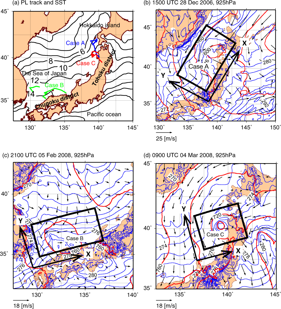
Fig. 1
(a) Sea surface temperatures (SSTs) (solid contours, every 2°C) averaged from December to March for the years 2003–2012, and the tracks of the examined PLs: case A (blue line), case B (green lines) and case C (red line). The X–Y coordinate system, geopotential height (red contours), potential temperature (blue contours) and horizontal wind (vectors) of each PL in the middle of its lifetime: (b) case A (geopotential height, every 60 m; potential temperature, every 2 K); (c) case B (geopotential height, every 20 m; potential temperature, every 1 K); (d) case C (geopotential height, every 20 m; potential temperature, every 1 K).
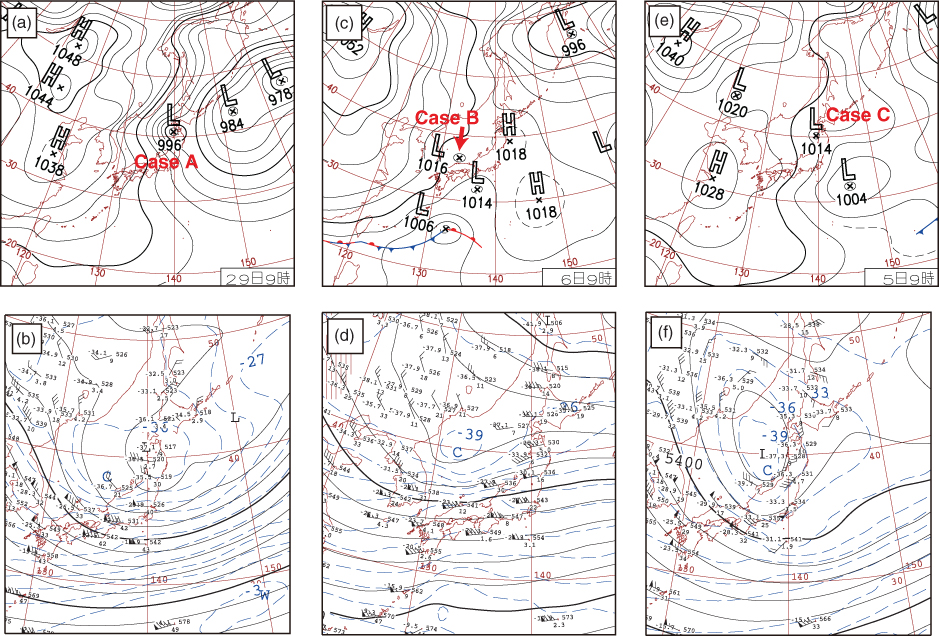
Fig. 2
Weather charts provided by the JMA: (a) Surface and (b) 500 hPa weather charts at 0000 UTC on 29 December 2006, (c) surface and (d) 500 hPa weather charts at 0000 UTC on 6 February 2008, and (e) surface and (f) 500 hPa weather charts at 0000 UTC on 5 March 2008.
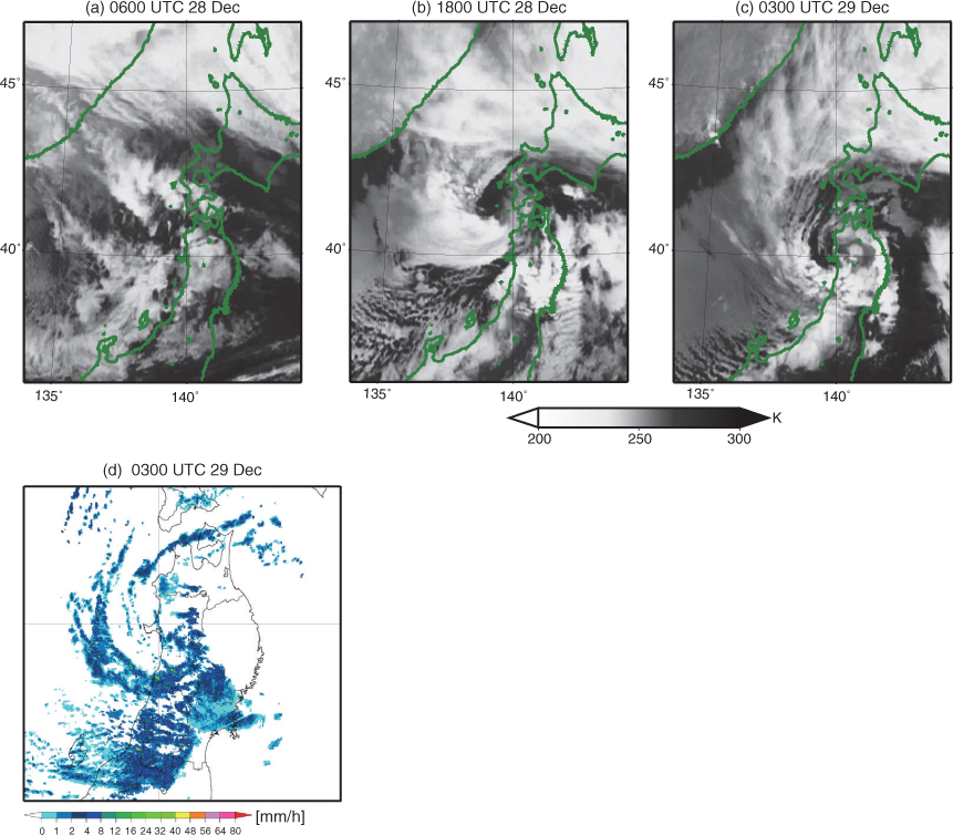
Fig. 3
Case A. Satellite images: (a) 0600 UTC on 28 December (incipient stage), (b) 1800 UTC on 28 December (development stage) and (c) 0300 UTC on 29 December 2006 (mature stage). (d) Radar composite image at 0300 UTC on 29 December 2006 (mature stage).
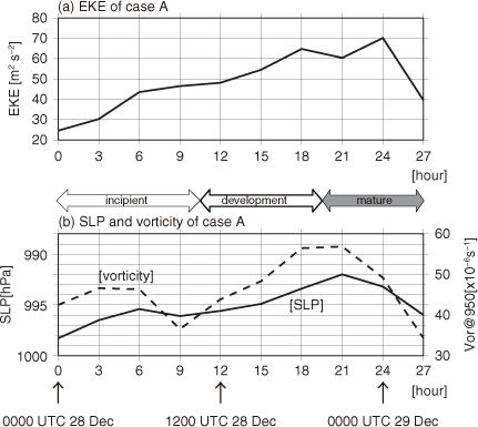
Fig. 4
Case A. Time evolution of parameters from 0000 UTC on 28 December to 0300 UTC on 29 December 2006: (a) EKE, averaged horizontally over the X–Y domain (see Fig. 1b) and vertically from 925 to 800 hPa. (b) Sea level pressure (SLP) at the PL centre (solid line), and relative vorticity, averaged horizontally over the X–Y domain at 950 hPa (dashed line).
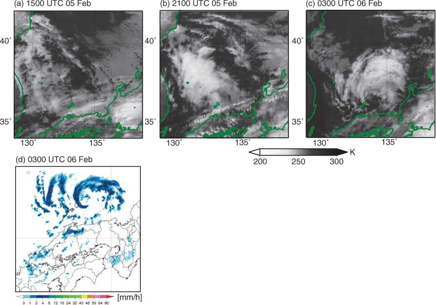
Fig. 5
Case B. Satellite images: (a) 1500 UTC on 5 February (incipient stage), (b) 2100 UTC on 5 February (development stage) and (c) 0300 UTC on 6 February 2008 (development stage). (d) Radar composite image at 0300 UTC on 3 February 2008 (development stage).
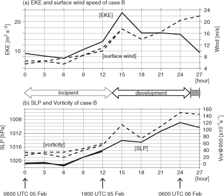
Fig. 6
Case B. Time evolution of parameters from 0600 UTC on 5 February to 0900 UTC on 6 February 2008: (a) EKE, averaged horizontally over the X–Y domain and vertically from 925 to 800 hPa (solid lines), and maximum surface wind (dashed lines). (b) SLP at the PL centre (solid lines) and maximum relative vorticity at 950 hPa (dashed lines; one for each incipient disturbance). Values at 1200 UTC on 6 February 2008 are excluded because half of the PL was outside of the X–Y domain.
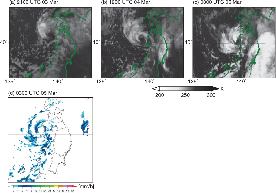
Fig. 7
Case C. Satellite images: (a) 2100 UTC on 3 March (development stage), (b) 1200 UTC on 4 March (development stage) and (c) 0300 UTC on 5 March 2008 (mature stage). (d) Radar composite image at 0300 UTC on 5 March 2008 (mature stage).
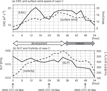
Fig. 8
Case C. Time evolution of parameters from 0600 UTC on 3 March to 1200 UTC on 5 March 2008: (a) EKE, averaged horizontally over the X–Y domain and vertically from 925 to 800 hPa (solid line), and maximum surface wind (dashed line). (b) SLP at the PL centre (solid line), and relative vorticity averaged within a 35 km radius of the centre at 975 hPa (dashed line).
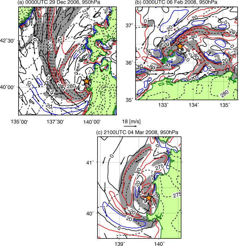
Fig. 9
Map views of potential temperature (dashed contours; every 1 K), upward wind (red contours, drawn at 20, 80 and 160 hPa h−1) and downward wind (blue contours, drawn at 20, 80 and 160 hPa h−1) at 950 hPa. (a) Case A at 0000 UTC on 29 December 2006 (mature stage); (b) case B at 0300 UTC on 6 February 2008 (development stage); and (c) case C at 2100 UTC on 4 March 2008 (mature stage). Shading indicates a horizontal gradient of potential temperature greater than 3 K per 100 km. W, warm core; vectors, horizontal wind; and orange star, PL centre. Vertical winds over land are masked out because of unrealistic and excessively high values (see subsection 2.1).
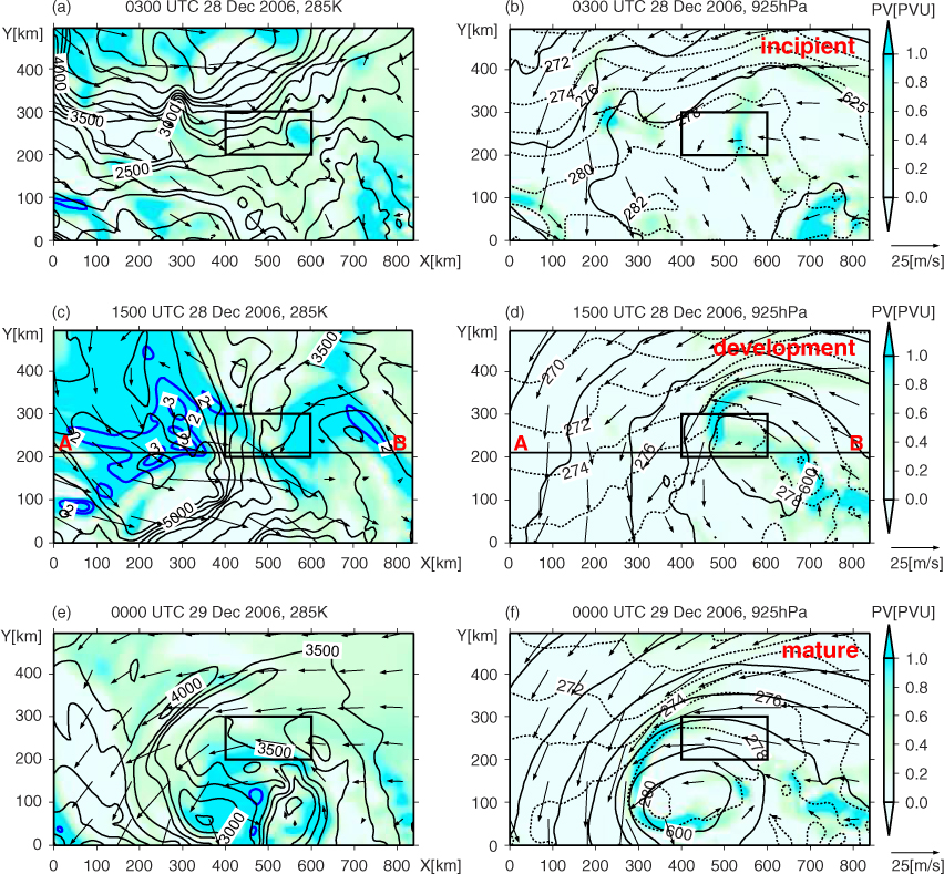
Fig. 10
Case A. Horizontal cross sections of the X–Y domain at 0300 UTC and 1500 UTC on 28 December and 0000 UTC on 29 December 2006: (a, c, e) at the 285 K isentropic surface, and (b, d, f) at 925 hPa. In panels (a), (c) and (e), PV is shown by blue shading with blue contours at intervals of 1.0 PVU (= 10−6m2 s−1 K kg−1). Black contours and vectors denote geopotential height (every 250 m) and horizontal wind, respectively. In panels (b), (d) and (f), solid contours, dotted contours, vectors and blue shading denote geopotential height (every 25 m), potential temperature (every 2 K), horizontal wind and PV (PVU), respectively. Bold rectangle shows the area of the incipient disturbance of case A. Line AB shows the location of the vertical cross section in Fig. 12.
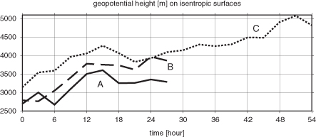
Fig. 11
Time evolution of geopotential height (m) on isentropic surfaces within the enclosed areas (bold rectangles or squares) shown in Fig. 10 (case A), 13 (case B) and 15 (case C). Solid line, case A (285 K isentropic surface); dashed line, case B (288 K); and dotted line, case C (285 K).
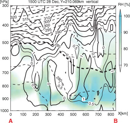
Fig. 12
Case A. Vertical cross section along the line AB shown in Fig. 10c and 10d at 1500 UTC on 28 December 2006: PV (thick contours, every 1.0 PVU), 0.5 PVU PV (thin contours), potential temperature (dashed contours, every 5 K), 285 K potential temperature (bolded dashed contour) and relative humidity (%) (blue shading).
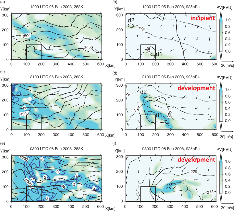
Fig. 13
Case B. Horizontal cross sections of the X–Y domain at 1200 UTC and 2100 UTC on 5 February and at 0300 UTC on 6 February 2008: (a, c, e) at the 288 K isentropic surface; and (b, d, f) at 925 hPa. In panels (a), (c) and (e), PV is shown by blue shading with blue contours at intervals of 1.0 PVU. Black contours and vectors denote geopotential height (every 250 m) and horizontal wind, respectively. In panels (b), (d) and (f), solid contours, dotted contours, vectors and blue shading denote geopotential height (every 25 m), potential temperature (every 2 K), horizontal wind and PV (PVU), respectively. In panel (b) and (d), two incipient disturbances d1 and d2 are also shown. Bold rectangle shows the area of the incipient disturbance d1 of case B.
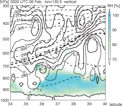
Fig. 14
Case B. Vertical cross section along 130.5°E (see Fig. 17b) at 0000 UTC on 6 February 2008: PV (thick contours, every 1.0 PVU), 0.5 PVU PV (thin contours), potential temperature (dashed contours, every 5 K), 288 K potential temperature (bold dashed contour) and relative humidity (%) (blue shading).
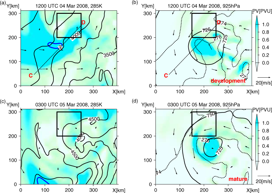
Fig. 15
Case C. Horizontal cross sections of the X–Y domain at 1200 UTC on 4 March and 0300 UTC on 5 March 2008: (a, c) at the 285 K isentropic surface, and (b, d) at 925 hPa. In panels (a) and (c), PV is shown by blue shading with blue contours at intervals of 1.0 PVU. Black contours and vectors denote geopotential height (every 250 m) and horizontal wind. In panels (b) and (d), solid contours, dotted contours, vectors and blue shading denote geopotential height (every 25 m), potential temperature (every 2 K), horizontal wind and PV (PVU), respectively. Bold rectangle shows the area of the incipient disturbance of case C. Line CD shows the location of the vertical cross section in Fig. 16.
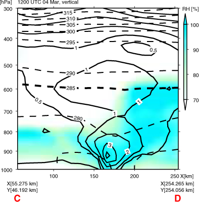
Fig. 16
Case C. Vertical cross section along the line CD in Fig. 15a and 15b at 1200 UTC on 4 March 2008: PV (thick contours, every 1.0 PVU), 0.5 PVU PV (thin contours), potential temperature (dashed contours, every 5 K), 285 K potential temperature (bold dashed contour) and relative humidity (%) (blue shading).
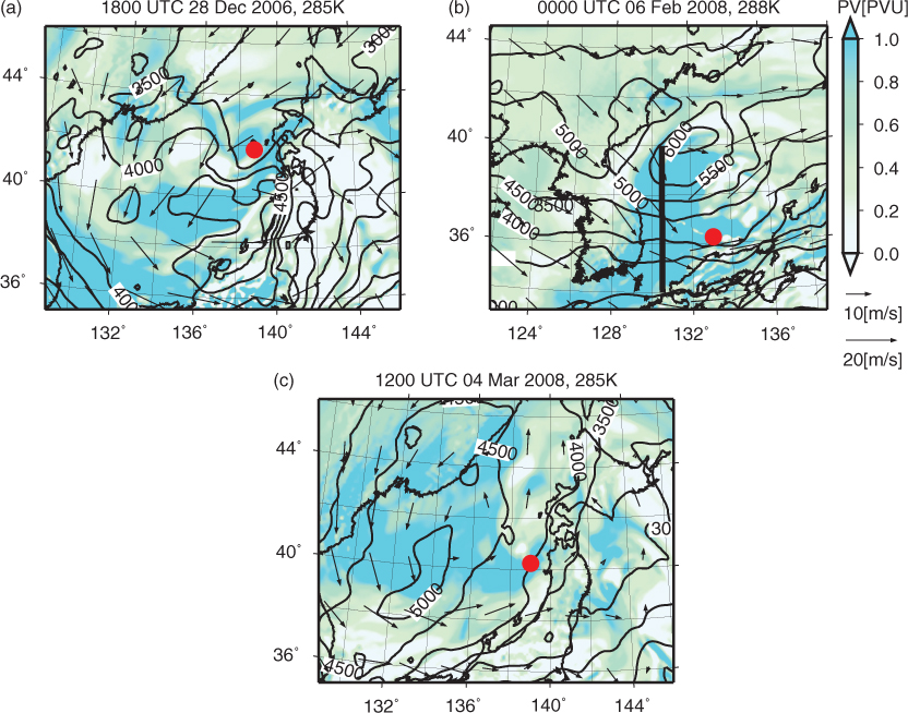
Fig. 17
Geopotential height (solid contours, every 250 m) and horizontal wind (vectors): (a) case A, 285 K isentropic surface at 1800 UTC on 28 December 2006 (development stage); (b) case B, 288 K isentropic surface at 0000 UTC on 6 February 2008 (development stage); and (c) case C, 285 K isentropic surface at 1200 UTC on 4 March 2008 (development stage). A red circle marks the centre of each PL, and shading indicates isentropic PV. Heavy straight line in (b) shows the location of the vertical cross section in Fig. 14.
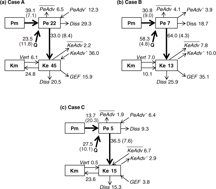
Fig. 18
Flow charts of the energy budgets showing EPE and EKE cycling. The numerals in boxes after Pe or Ke indicate the energy (m2 s−2) averaged horizontally over each X–Y domain over the incipient and development stage of each PL, and vertically from 925 hPa to 800 hPa. Numerals next to the arrows are energy conversion rates (10−6 s−1) normalised by the averaged Ke, averaged horizontally over the X–Y domain over the incipient and development stage of each PL, and vertically from 925 hPa to 800 hPa. Numerals in parentheses are the reciprocals of the Ke-normalised energy conversion rates (hour): (a) case A (averaged over the period from 0000 UTC on 28 December to 1800 UTC on 29 December 2006); (b) case B (averaged over the period from 0600 UTC on 5 February to 0600 UTC on 6 February 2008); and (c) case C (averaged over the period from 0600 UTC on 3 March 2008 to 1500 UTC on 4 March 2008).
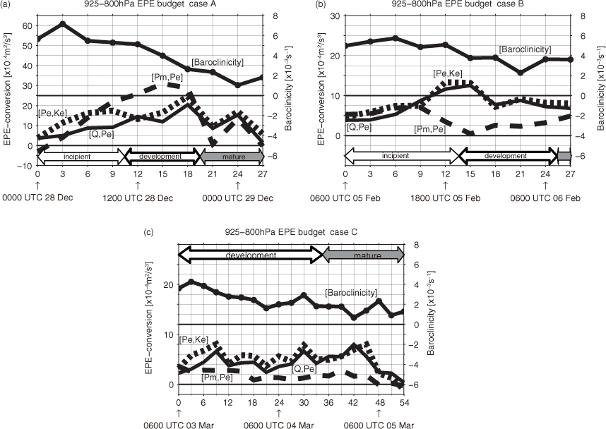
Fig. 19
Time evolution of [Pm, Pe] (dashed line), [Q, Pe] (thin solid line), [Pe,Ke] (dotted line) and baroclinicity (thick solid line with circles) averaged over each X–Y domain. Unlike the values in Fig. 18, these values are not normalised. (a) Case A; (b) case B; (c) case C.
Table 1. Characteristics of the three PLs of cases A, B and C
Rossby height, H R 4580 m4380 m2510 mScale of the intruding UPV anomaly, L300 km300 km150 kmLocation of the cold vortex at 500 hPa during the mature stageImmediately above the PL400 km north of the PLImmediately above the PLBaroclinicityStrong→weakStrongStrong→weakCloud patternComma-shaped→spiraliformComma-shapedComma-shaped→spiraliformDominant development processBaroclinicDiabaticDiabaticMagnitude of EKELargeSmallSmall