
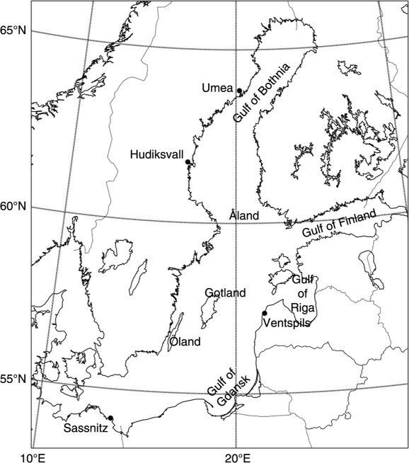
Fig. 1
A map of the Baltic Sea region highlighting areas referred to in this study.
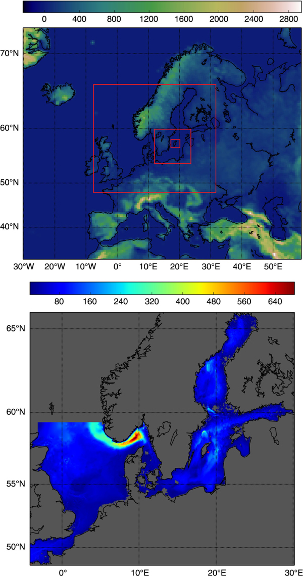
Fig. 2
(a) WRF domains and (b) NEMO domain. The outer WRF domain has a horizontal resolution of 30 km, and each nest has a grid refinement factor of 3. NEMO has a horizontal resolution of 2 nm. Topography (WRF, metres) and bathymetry (NEMO, metres) are shaded.
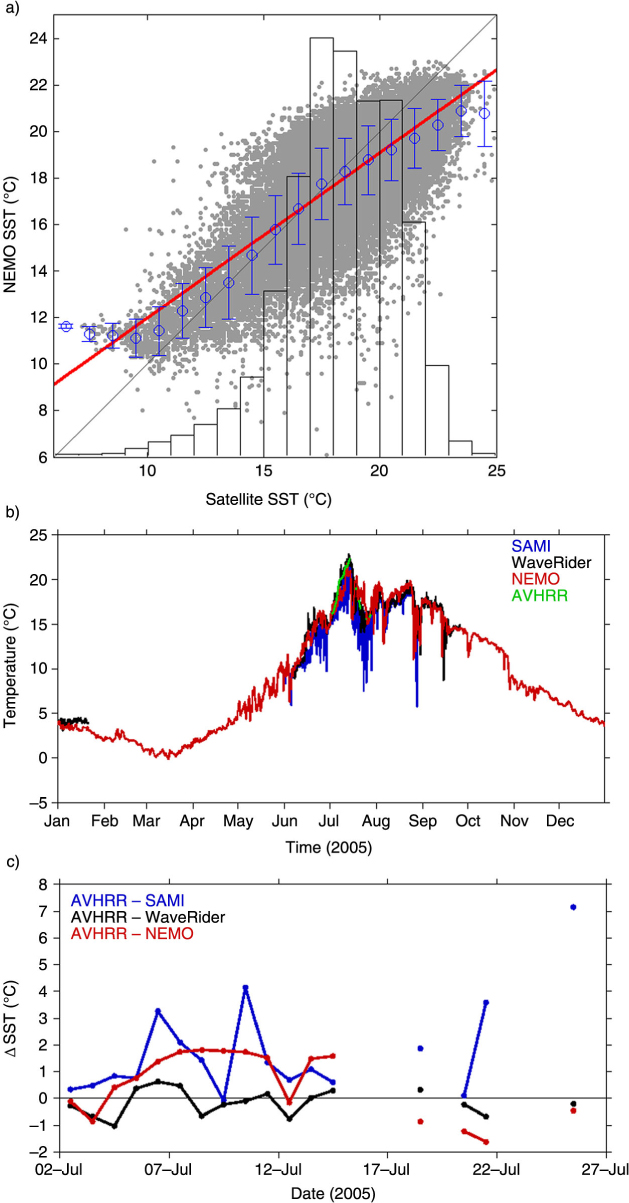
Fig. 3
(a) A point-wise comparison of simulated and satellite sea-surface temperature for July 2005 over the Baltic Sea. The red line shows the linear fit and the blue bars show 1°C bin averages with standard deviation. Black bars show the normalised distribution of satellite SST. (b) A timeseries of SST at the Östergarnsholm observation site, for 2005, showing NEMO (red), waverider (black), SAMI (blue) and AVHRR (green) SSTs, where available. (c) The difference between remotely sensed and in-situ/modelled data, where all are available.
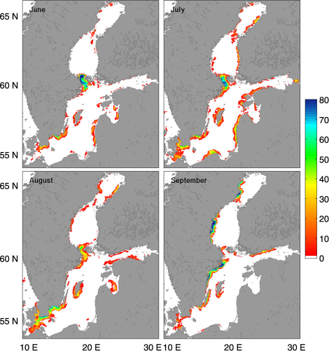
Fig. 4
The frequency of upwelling with a detectable SST signature for the months of June, July, August and September, 2005 (%).
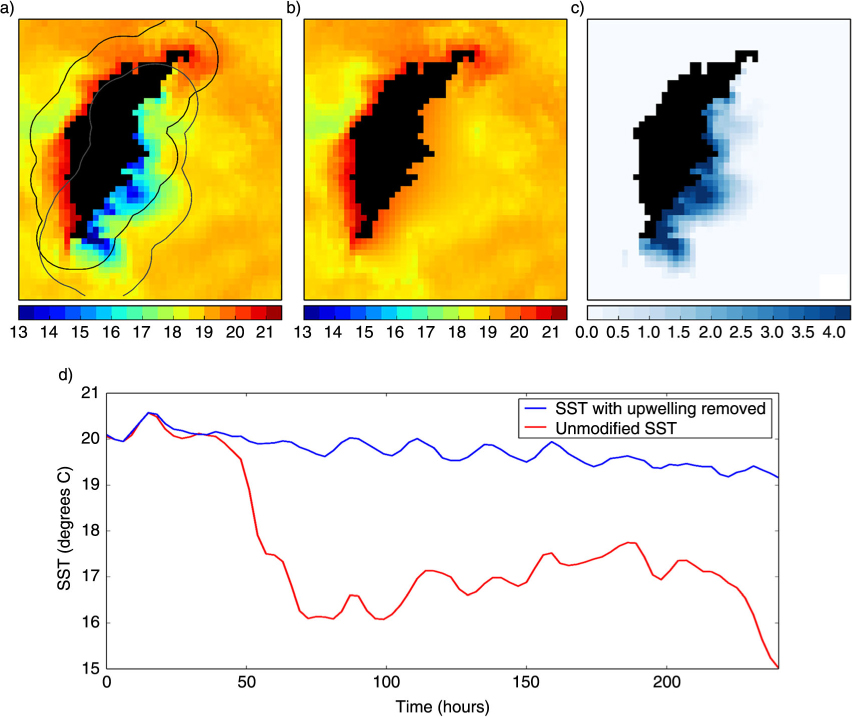
Fig. 5
Detection and removal of upwelling. The left panel (a) shows the modelled SST (°C), with a strong upwelling event along the south-east coast of Gotland. The black line indicates the area around the coast where upwelling is initially detected, and the thick grey line where the secondary search is carried out. The thin grey line shows the identified area of upwelling-modified water. The middle panel (b) shows the same SST as the left, but with the upwelling region interpolated over. The right panel (c) shows the difference between the upwelling and no-upwelling cases. The timeseries (d) shows temperature evolution in the upwelling (blue) and no-upwelling (red) simulations get the Östergarnsholm measurement site.
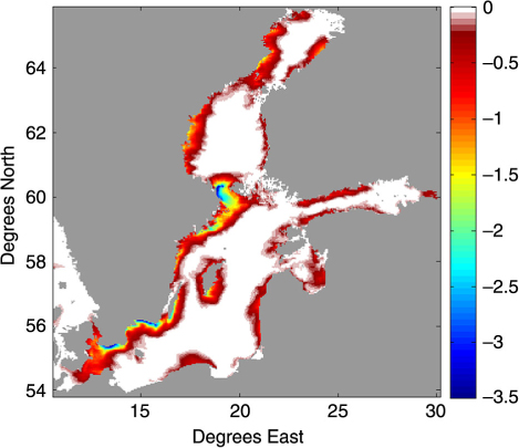
Fig. 6
The mean summer (June–September) sea-surface temperature (°C) difference (no-upwelling–upwelling) between the standard model SST and the model SST which has had the upwelling signature removed at every output time.
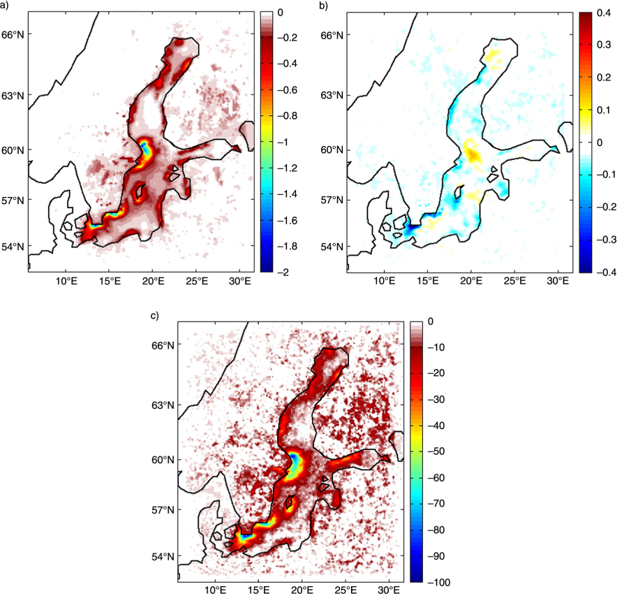
Fig. 7
Composite differences between upwelling and no-upwelling simulations, averaging from June through September 2005. (a) 2 m temperature (°C); (b) 10 m wind speed (m s−1), (c) boundary-layer height (m).
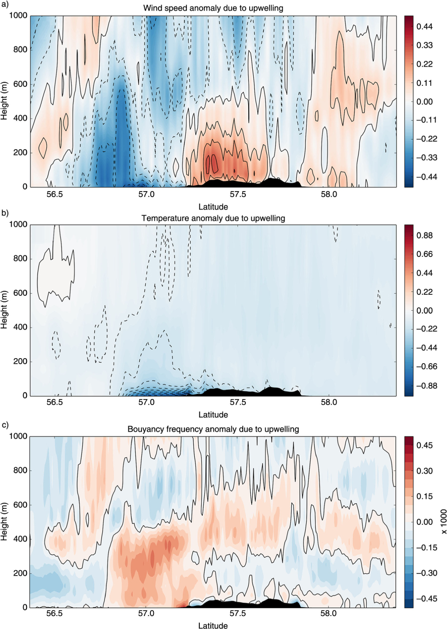
Fig. 8
Cross-sections (mean from 18°E to 19.5°E) of differences in wind speed (a); potential temperature (b); and buoyancy frequency (c) due to upwelling during an upwelling event in July 2005.
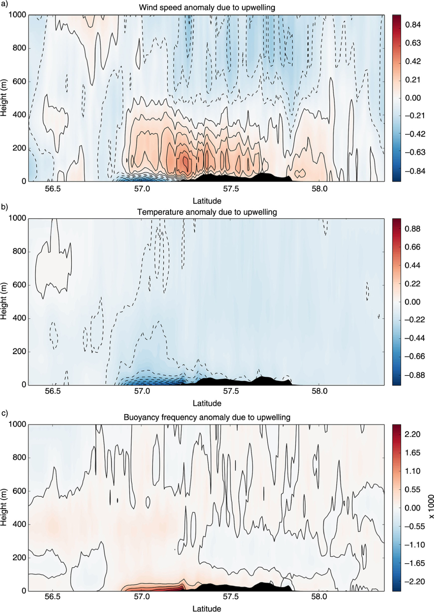
Fig. 9
Cross-sections (mean from 18°E to 19.5°E) of differences in wind speed (a); potential temperature (b); and buoyancy frequency (c) due to upwelling during an upwelling event in July 2005, where the strength of the upwelling (temperature deviation from no-upwelling simulation) has been doubled.
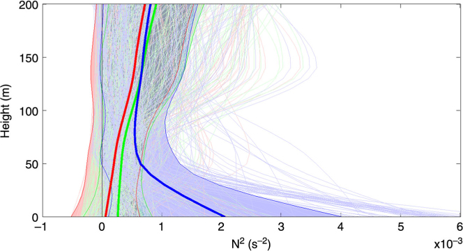
Fig. 10
Profiles of the square of buoyancy frequency in the lower boundary layer off the south-east coast of Gotland during the July 2005 upwelling period for no-upwelling (red), upwelling (green) and 2×upwelling (blue). Thin lines show profiles at every 3 hours, and thick lines show the mean over the simulation. Shaded areas show ±one standard deviation from the mean.