
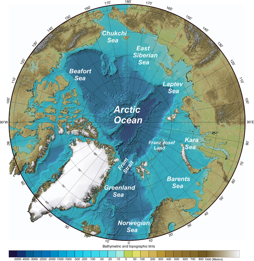
Fig. 1
Arctic Ocean.
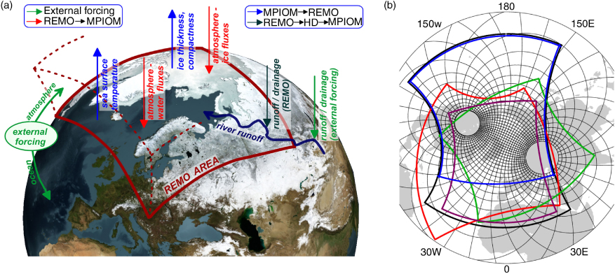
Fig. 2
MPIOM/REMO/HD Coupling (a) and coupled setups (b). Coloured spherical rectangles on (b): Arctic (violet), Asia (green), Atlantic (red), Pacific (blue), Atlantic–Pacific (black). Domains are defined on REMO grid. Thin black lines – MPIOM grid (every 12th grid line).
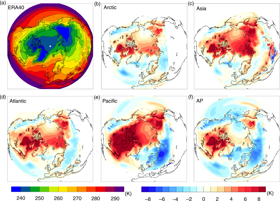
Fig. 3
Mean (1958–2001) ERA40 DJF 2 m temperature and difference Model – ERA40 [K].
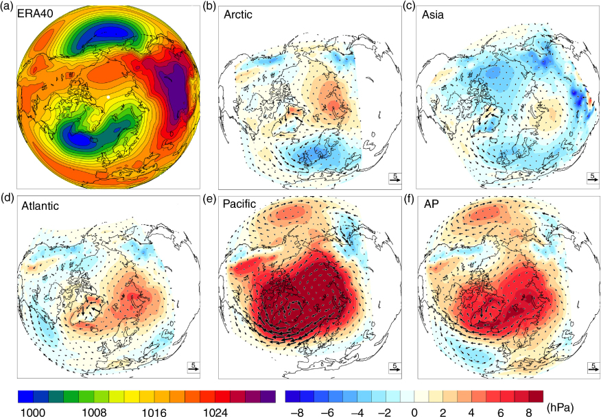
Fig. 4
Mean (1958–2001) ERA40 DJF sea level pressure and difference Model – ERA40 [hPa]. Vectors show the anomalous circulation induced in terms of 10 m wind speed (Model – ERA40). Arrow in the right corner – reference vector (5 m/s)
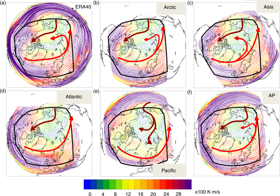
Fig. 5
Mean DJF 500 hPa heat transport (v·T) [100 K·m/s] calculated from 6-hourly temperature and wind velocity. Black polygon indicates the common part of all the five setups. Thick arrows schematically represent the Atlantic (red arrows) and Pacific (brown arrows) atmospheric flow.
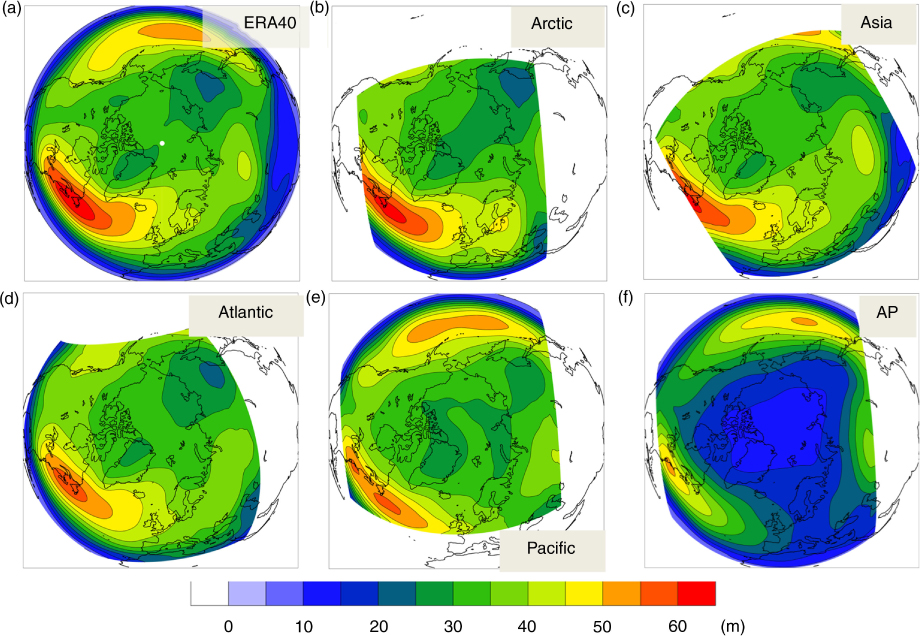
Fig. 6
Storm track calculated as a standard deviation of bandpass (2.5 – 6 d) filtered DJF 500 hPa geopotential height (m), see main text for more details.
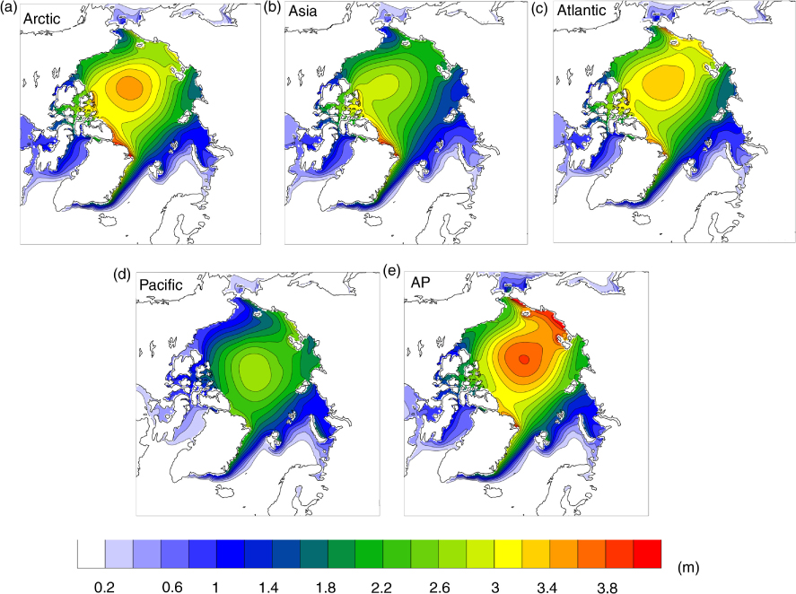
Fig. 7
Mean DJF sea ice thickness [m].
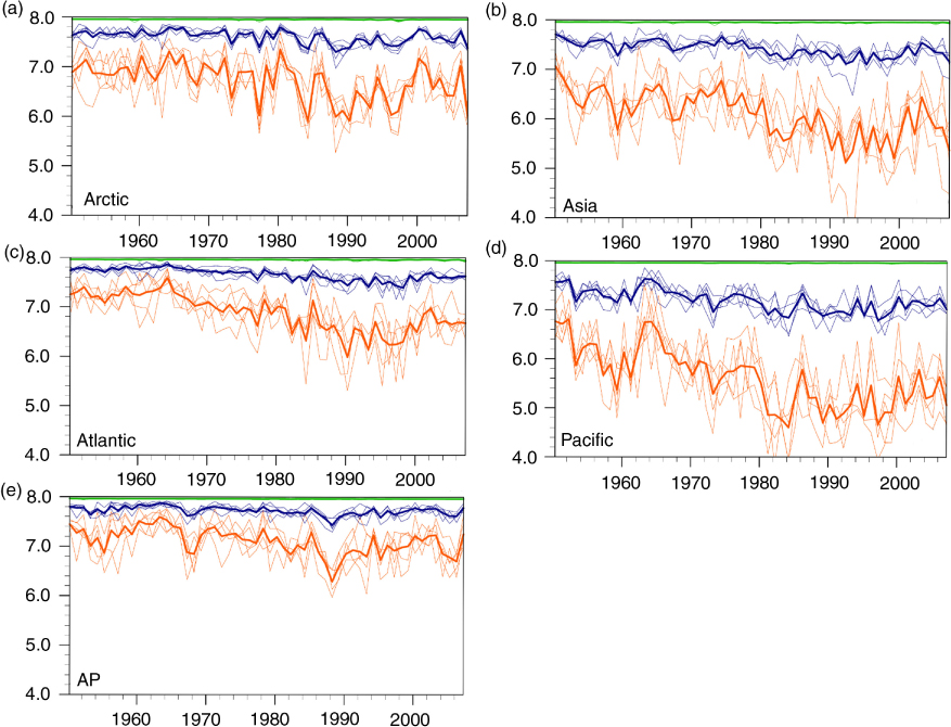
Fig. 8
Sea ice area in Arctic Ocean (x106 km2): March (green), September (red), Annual mean (blue). Thin solid lines – ensemble members, thick solid lines – ensemble means, black dashed lines – observations for corresponding months (Cavalieri et al., 1996).
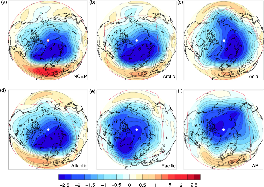
Fig. 9
Leading EOF of DJF MSLP anomalies over NH (20°–90°N), red spherical rectangles indicates the coupled area.
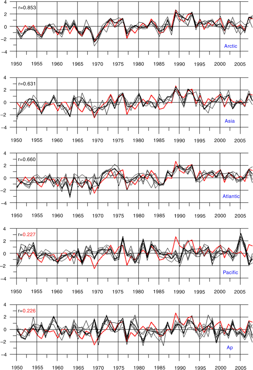
Fig. 10
Normalised principal components of the leading EOF of DJF MSLP anomalies (hPa) over NH (20°–90°N) Black thin lines – ensemble members. Black thick line – ensemble mean. Red line – those calculated from NCEP/NCAR MSLP. The numbers on time series plots: correlation between ensemble means and reanalysis, that is, thick black and red line.
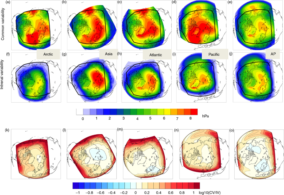
Fig. 11
Mean DJF common (upper row) and internal (centre row) sea level pressure variability. The black polygon indicates the common area of all the five coupled domains. Lower row: log10 of relative variability [common (CV) divided by internal (IV)].
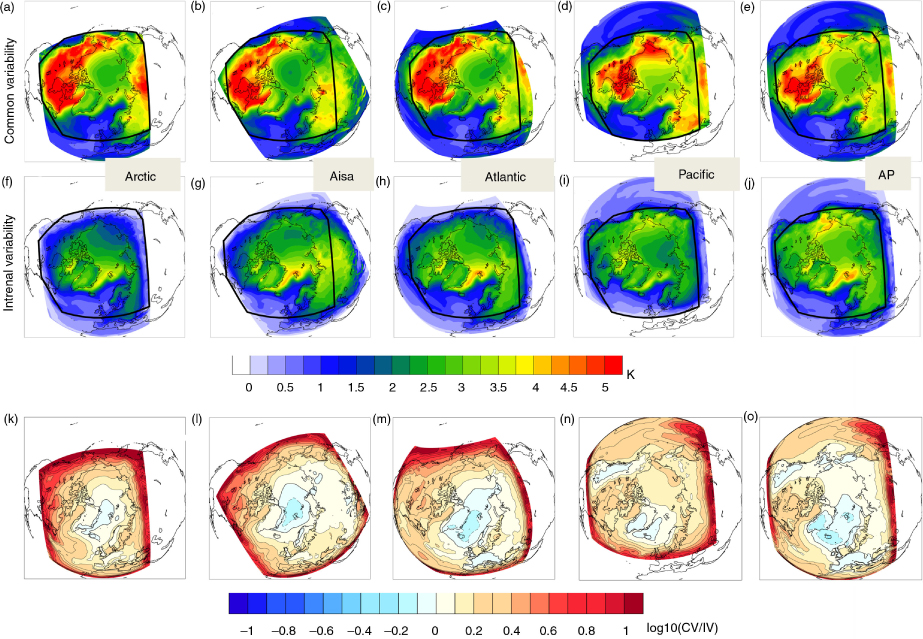
Fig. 12
Mean DJF common (upper row) and internal (centre row) 2 m temperature variability. The black polygon indicates the common area of all the five coupled domains. Lower row: log10 of relative variability [common (CV) divided by internal (IV)].
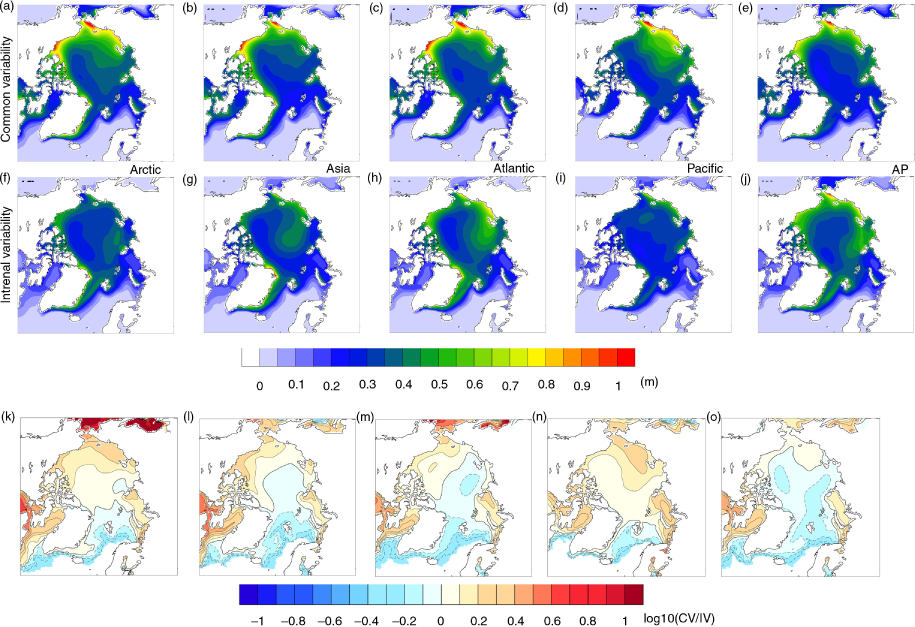
Fig. 13
Mean DJF sea ice thickness common variability (upper row) and internal variability (centre row). Lower row: log10 of relative variability [common (CV) divided by internal (IV)].