
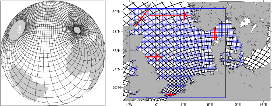
Fig. 1
Left panel: grid configuration of the MPIOM global model experiment (every 12th grid line is shown). Right panel: grids (every 5th grid line is shown for both models) in the North Sea for the MPIOM global model experiment (black lines) and HAMSOM regional model experiment (blue lines, resolution ~3 km). The thick blue square marks the area covered by BSH satellite SST data. The red lines and arrows indicate the main current direction for different sections.
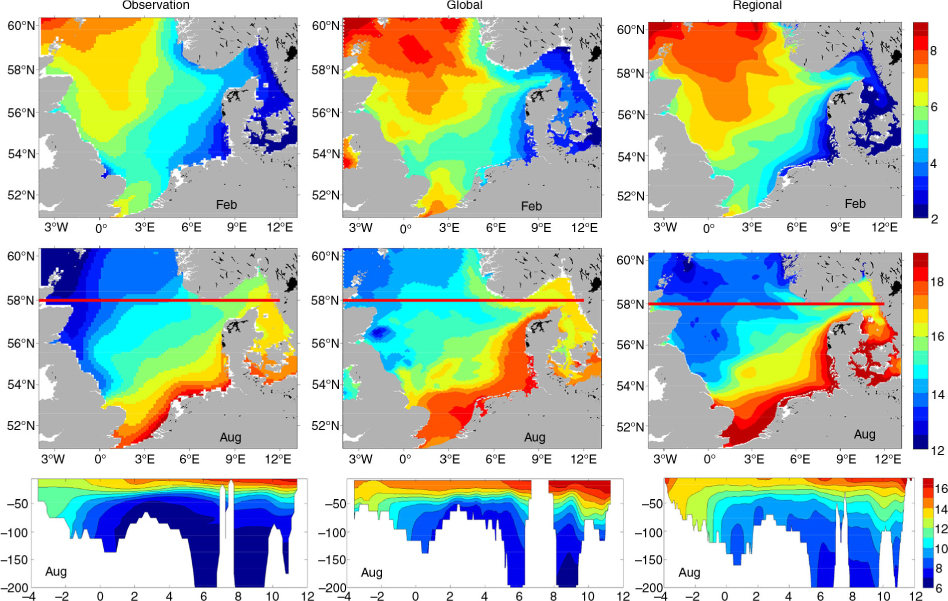
Fig. 2
Climatological SST (upper panels) and vertical temperature distribution at section 58°N (bottom panels) in February and August of observations (Janssen et al., 1999, left column), MPIOM global (middle column) and HAMSOM regional (right column) simulations. Red lines mark the location of the section at 58°N.
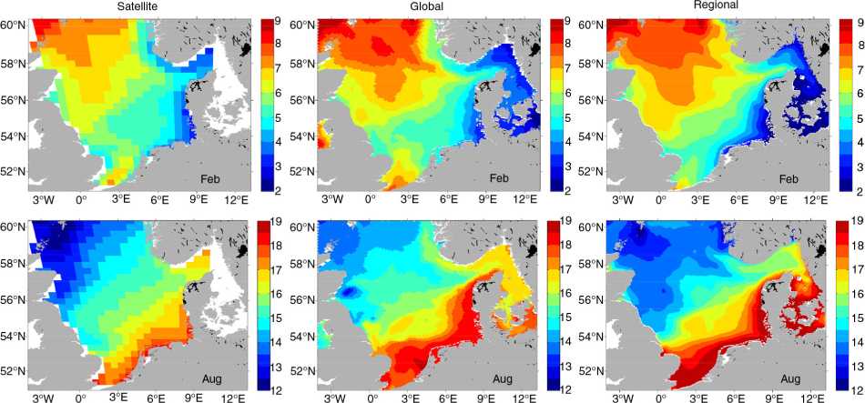
Fig. 3
Mean of 22 yr SST (1979–2000) in February (upper panel) and August (bottom panel) of satellite observations (left column), MPIOM global (middle column) and HAMSOM regional (right column) simulations.
Table 1. Annual mean transport estimations from MPIOM, HAMSOM, HYCOM and measurements
Orkney-Shetland inflow0.530.570.490.30English Channel inflow0.190.080.160.1–0.17Norwegian channel outflow1.491.322.331.8Shetland shelf inflow0.730.660.50.6Skagerrak inflow0.420.811.020.5–1.5Skagerrak outflow0.440.841.040.5–1.5Eastern British coastal currents0.010.1
[i] The sections are illustrated in Fig. 1. HYCOM results and measurements are taken from Winther and Johannessen (2006) and references therein. All values are given in Sv (1 Sv = 106 m3 s−1).
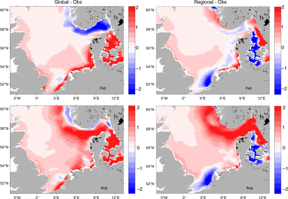
Fig. 4
Left column: difference between Climatological SSS (psu) in February and August between observations (Janssen et al., 1999) and MPIOM global simulations (MPIOM minus observations). Right column: SSS difference between observations and HAMSOM regional simulations (HAMSOM minus observations).
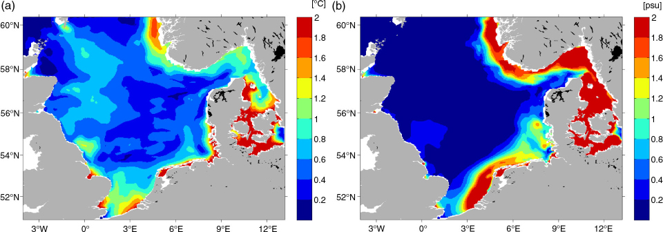
Fig. 5
Root mean square difference of SST and SSS between MPIOM and HAMSOM model results. (a) RMSD SST; (b) RMSD SSS.
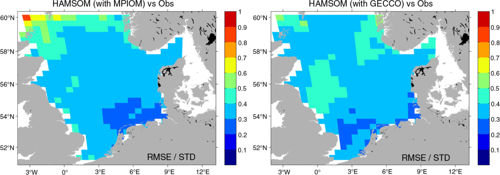
Fig. 6
The ratio of root mean square error (RMSE) to standard deviations of BSH SST data. RMSE is calculated between HAMSOM simulations with open boundary forcing from MPIOM (left) and from GECCO (right) and BSH SST observations (weekly), and only for the years 1979–2000 (data period).
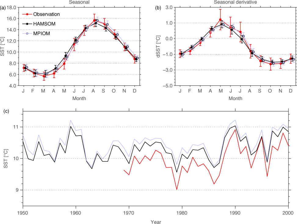
Fig. 7
(a) Seasonal cycle of spatially averaged climatological monthly mean SST for the North Sea, error bars denote the standard deviation. (b) Derivative of monthly mean SST (monthly mean SST minus previous monthly mean SST), error bars denote the standard deviation. (c) The inter-annual variability of spatially and yearly averaged SST over the North Sea. Grey and black lines refer to the results from MPIOM and HAMSOM, respectively. The red lines refer to observations.
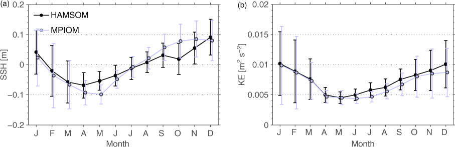
Fig. 8
Spatially averaged climatological monthly means (lines) and standard deviations (error bars) of SSH (a) and kinetic energy (b). The grey colour refers to the MPIOM results, the black colour to the HAMSOM results.
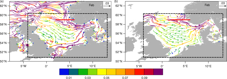
Fig. 9
Climatological surface current fields (m s−1) of (a) MPIOM and (b) HAMSOM (upper 15 m) results for February. The colours refer to current speeds (m s−1). The black dashed line shows the domain of HAMSOM model, and the red thick lines refer to 59°N section in Fig. 10.
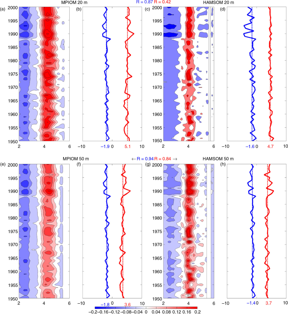
Fig. 10
(a, c, e, g) Hovmöller Diagram of meridional current speeds (m s−1) in February at 20 m (upper panel) and 50 m depth (bottom panel) through the 59°N section from 2°E to 6°E (location in Fig. 9) of MPIOM (left panel) and HAMSOM (right panel) model results. Blue indicates the southward, and red indicates the northward current. (b, d, f, h) The blue and red solid lines refer to the simple sum of the current speeds across the section, respectively. The correlation coefficients between both model results at 20 m depth are R = 0.87 (southward current) and R = 0.42 (northward current), and at 50 m depth are R = 0.94 (southward current), R = 0.84 (northward current). The mean north- and southward currents are presented by the dashed lines with their values (m s−1) noted at the x-axis of b, d, f, h.