
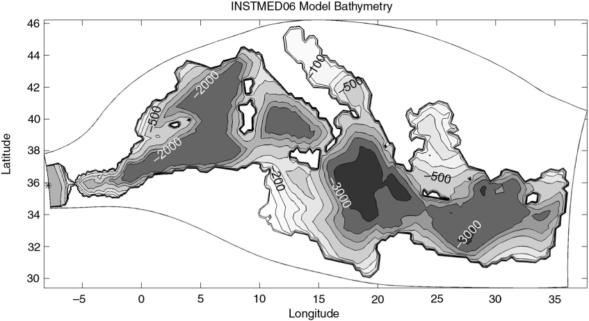
Fig. 1
Bathymetry used for the INSTMED06 Mediterranean Basin model. OTIS sea-level height tidal predictions used to force the INSTEMD06 are located at the first longitudinal grid point (7.9°W; 35.83°N) indicated by the ‘*’ sign.
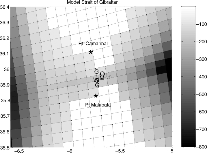
Fig. 2
Detailed bathymetry shown in Fig. 1 for the Strait of Gibraltar. The model grid is also plotted. The model has three grid points at the narrowest north–south section of the Strait. The locations of GE (velocity, temperature and salinity) and WOCE (velocity) measurements are shown by ‘G’ and ‘W’ letters, respectively; the location of tide currents from OTIS predictions is shown by the ‘O’ letter. The ‘M’ letter indicates the model grid point where the simulated temperatures and salinity are diagnosed. The arrow indicates the location where the simulated velocity is diagnosed. Density is derived at location ‘G’ for GE observations and ‘M’ for the model. The simulated volume transport through the Strait is calculated at the section crossed by the arrow.
Table 1. Summary of datasets used and simulations performed
GEDataOctober 22, 1985 at 16:00 to April 21, 1986 at 07:00Along-strait water velocity and water densityWOCE1DataNovember 8, 1994 at 17:00 to April 3, 1995 at 17:00Along-strait water velocitySTIGESimulation with tideJanuary 1, 1985 at 00:00 to April 21, 1986 at 07:00Varying atmospheric forcing
Tide forcingSNTW1Simulation without tideJanuary 1, 1994 at 17:00 to April 3, 1995 at 08:00.Varying atmospheric forcing
No tide forcingSTIW1Simulation with tideVarying atmospheric forcing
Tide forcingSTAW1Simulation with tide aloneConstant atmospheric forcing
Tide forcingSNT50Long simulation without tide50-yr: 1958–1967Varying atmospheric forcing
No tide forcingSTI50Long simulation with tideVarying atmospheric forcing
Tide forcingSNT20Short simulation without tide20dVarying atmospheric forcing
No tide forcingSTI20Short simulation with tideVarying atmospheric forcing
Tide forcingSNTS20Short simulation without tide; T, S smoothingVarying atmospheric forcing
No tide forcing
Smoothed T and S at Gibraltar
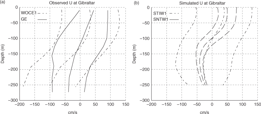
Fig. 3
Profiles of flow velocity at the Strait of Gibraltar (locations are shown in Fig. 2) with plus and minus one standard deviation. a) dashed–dotted lines: based on the WOCE1 measurements; continuous lines: based on the GE measurements. b) dashed–dotted lines: based on the simulation STIW1; dashed lines: based on the simulation SNTW1.
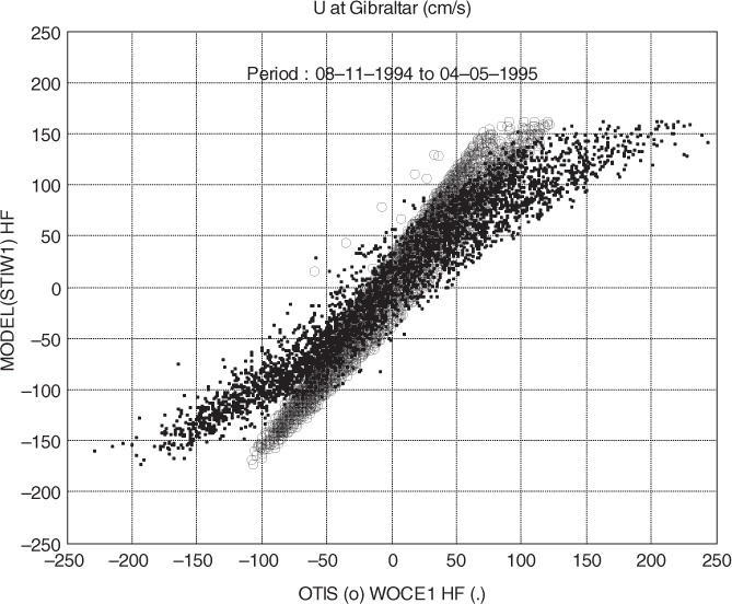
Fig. 4
Scatter plot of the high-pass filtered velocity at the Strait of Gibraltar (locations are shown in Fig. 2). Circles represent simulated velocities versus predicted ones using OTIS. Dots represent simulated velocities versus velocities based on the first WOCE sub period measurements. The simulation is STIW1 and the period considered is November 8, 1994 at 17:00 to April 3, 1995 at 08:00.
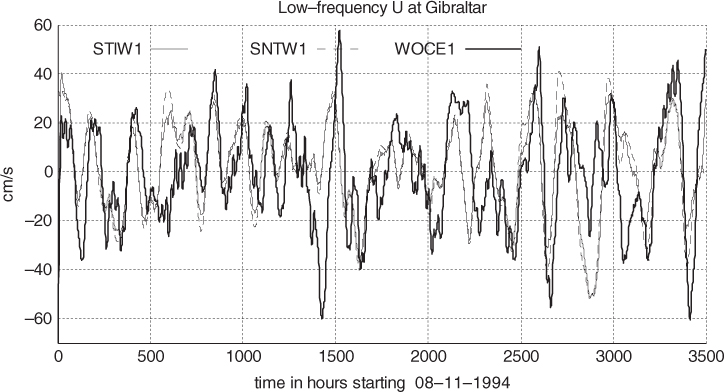
Fig. 5
Time series of the low-pass filtered velocity at the Strait of Gibraltar (locations are shown in Fig. 2). Continuous thick line: WOCE1 data first observing period. Continuous thin line: model simulation using tide as forcing at the Atlantic side (STIW1). Dashed thin line: model simulation without using tide as forcing (SNTW1). The period considered is November 8, 1994 at 17:00 to April 3, 1995 at 08:00.
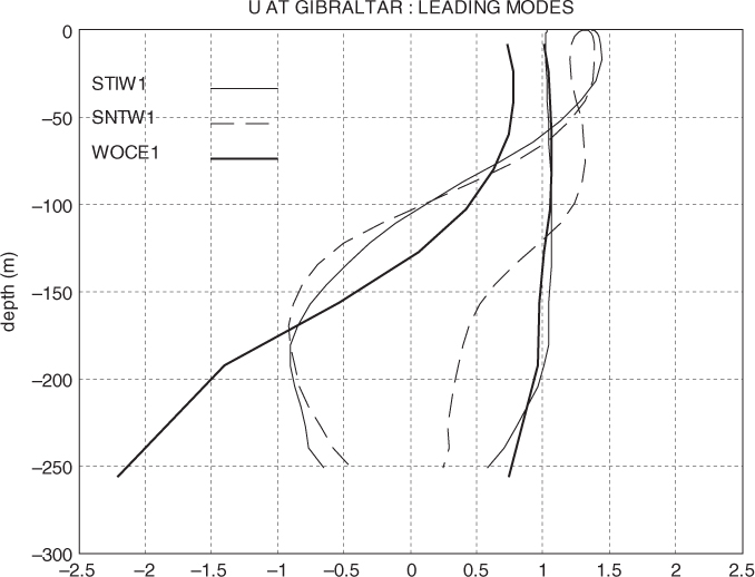
Fig. 6
Vertical profiles of the two derived modes of velocity at the Strait of Gibraltar (locations are shown in Fig. 2). Thick-continuous line: based on WOCE1 sub period measurements. Thin-continuous line: based on the simulation STIW1; thin-dashed line: based on the simulation SNTW1. The period is November 8, 1994 at 17:00 to April 3, 1995 at 08:00. Vertical profiles are standardised (rms=1).
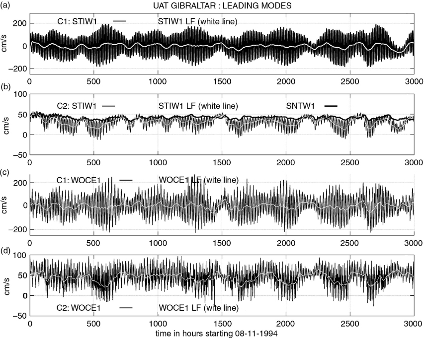
Fig. 7
Time series of velocity at the Strait of Gibraltar. a) hourly (black line) and low-pass filtered (white line) first-mode time series from STIW1. b) hourly (black line) and low-pass filtered (white line) second-mode time series from STIW1. The low-pass filtered second-mode from SNTW1 is also shown as thick black line. c) hourly (black line) and low-pass filtered (white line) first-mode time series from WOCE1. d) hourly (black line) and low-pass filtered (white line) second-mode time series from WOCE1. The period considered is November 8, 1994 at 17:00 to April 3, 1995 at 08:00.
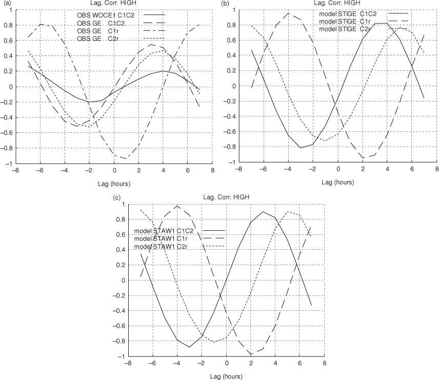
Fig. 8
Lagged correlations between selected observed and simulated series high-pass filtered to focus on the tidal oscillations at the M2 time scale. The abscissa are leading and lagging hours. a) based on observations using WOCE1 and GE data; b) based on the simulation STIGE; c) based on the tide-alone simulation STAW1. Negative abscissa corresponds to the case that the second variable leads the first variable, and the opposite is for positive abscissa. Legends indicate each pair of time series involved in the calculation. C1 and C2 refer to the first and second modes of velocity at the Strait and r to the mean density at the Strait.
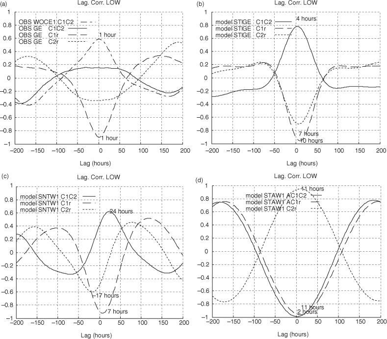
Fig. 9
Same as Fig. 8 but for selected observed and simulated series low-pass filtered to focus on the subinertial variability. a) based on observations using WOCE1 and GE data; b) based on the simulation STIGE; c) based on the simulation without tide SNTW1; d) based on the simulation where only tide is considered as a forcing STAW1. In d) the absolute value AC1 of the first mode C1 is used for correlations.
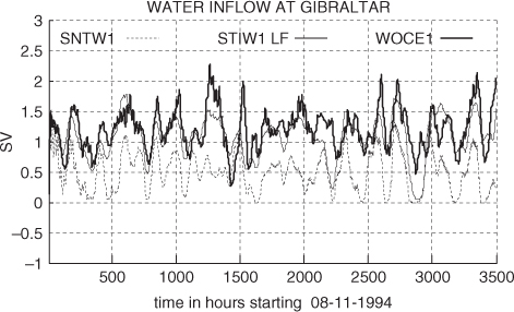
Fig. 10
Water fluxes into the Mediterranean basin through the Strait of Gibraltar. The simulated fluxes with tide STIW1 (continuous line) and without SNTW1 (dotted line) are shown. The water flux into the Mediterranean basin from WOCE1 is shown by a thick line. When calculating the fluxes into the Mediterranean basin, negative velocities are set to zero.
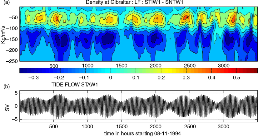
Fig. 11
a) low-pass filtered difference of density (kgm-3) at the Strait of Gibraltar between simulations STIW1 and SNTW1. The figure is shown as a time-depth Hovmöller diagram. b) for time reference, tide flow is shown as the mean water transport from the simulation where only tide is considered as forcing (STAW1, in Sv).
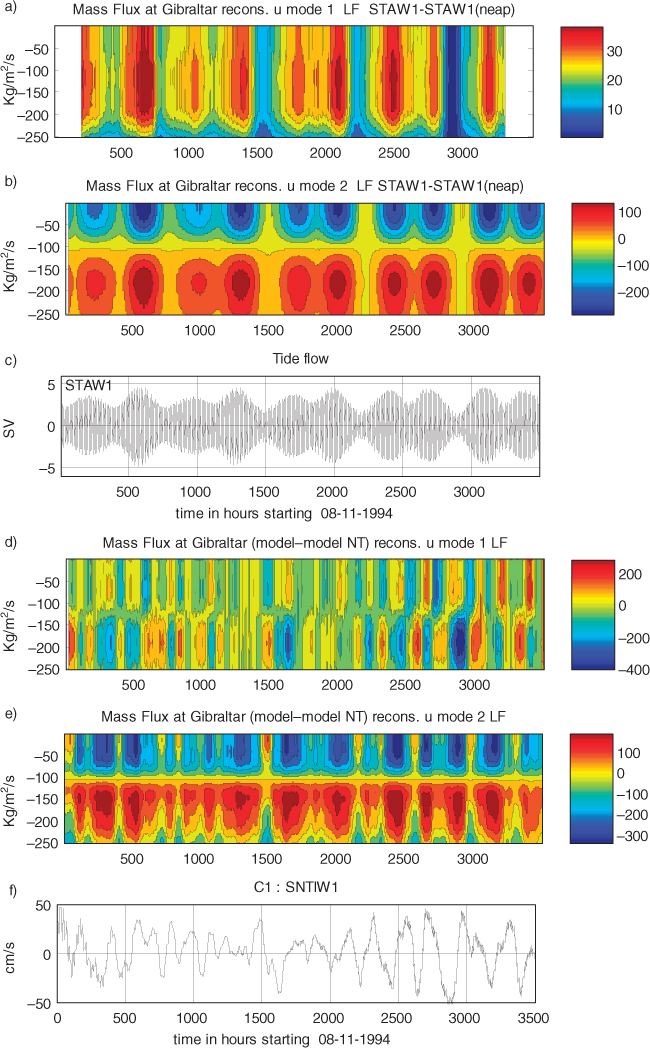
Fig. 12
a) mass flux through the Strait of Gibraltar (in kg m−2 s−1) reconstructed using the first mode of velocity low-pass filtered based on the simulation with tide alone (STAW1). The vertical profile for a neap tide state (the vertical profile at time number 2919) is subtracted to obtain deviations relative to an almost no tide state (the neap tide state). b) as a) but for the second mode. c) for time reference, the tide flow is shown as the mean water transport from the simulation where only tide is considered as forcing (STAW1). d) Difference of mass flux reconstructed with mode 1 of velocity between the tidal (STIW1) and no tidal (SNTW1) simulations, low-pass filtered (in kg m−2 s−1). e) as d) but for mode 2. f) for time reference, the subinertial flow induced by external forcing (first velocity mode from SNTW1, in cm/s).
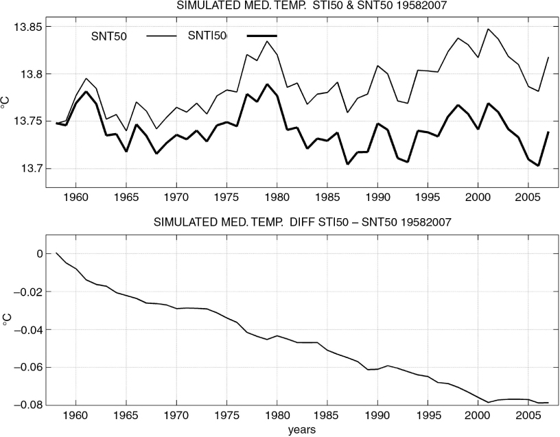
Fig. 13
Upper panel: Potential temperature averaged over the entire Mediterranean volume from the 50-yr simulations. Thick curve: tide is used as forcing; thin curve: without tide. Lower panel: their difference.
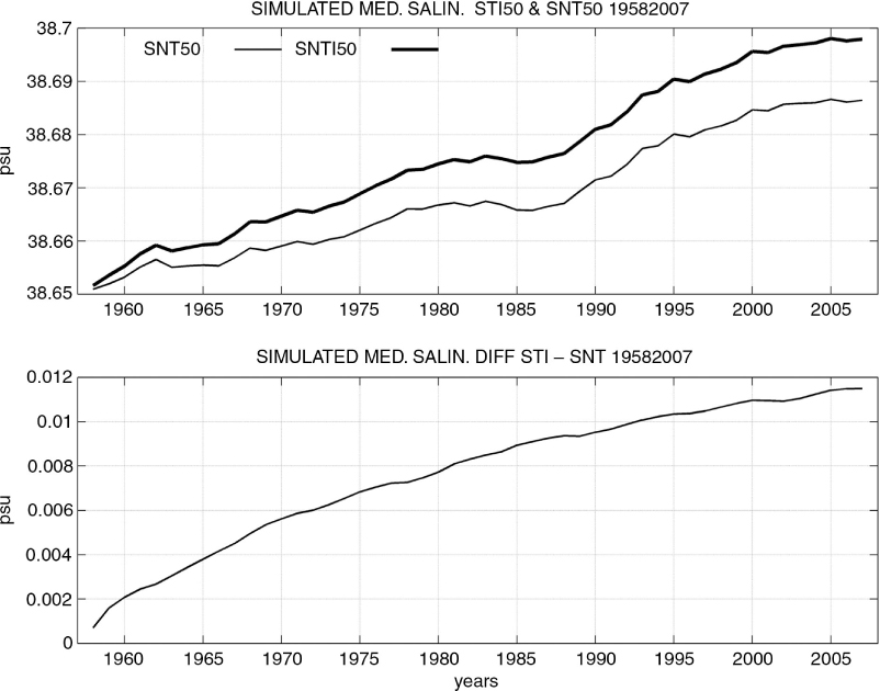
Fig. 14
Same as in Fig. 13 but for the average salinity.
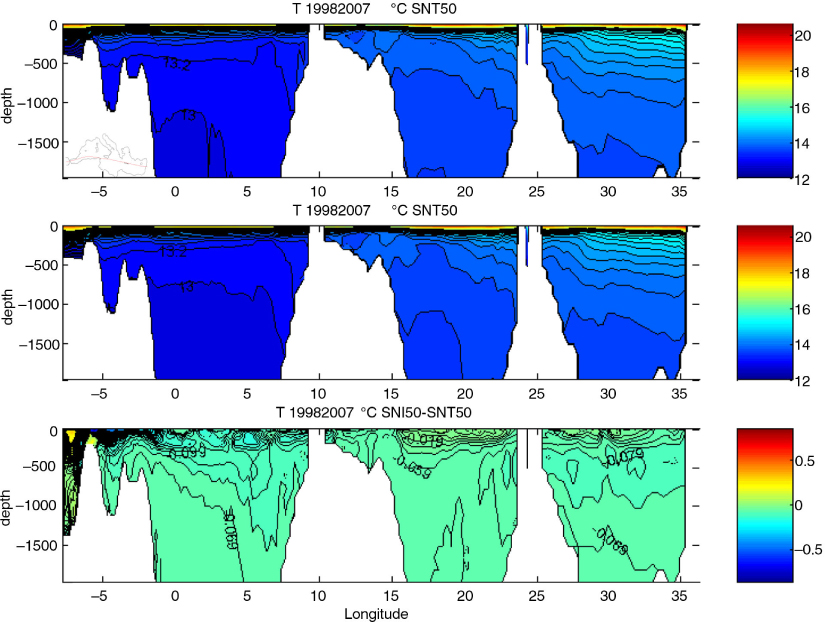
Fig. 15
Average potential temperature over the 10-yr period 1998–2007 from simulations STI50 (upper panel) and SNT50 (middle panel) and their differences (lower panel). Panels are shown along east–west vertical sections. The horizontal location of the section is presented on the lower left corner of the upper panel.
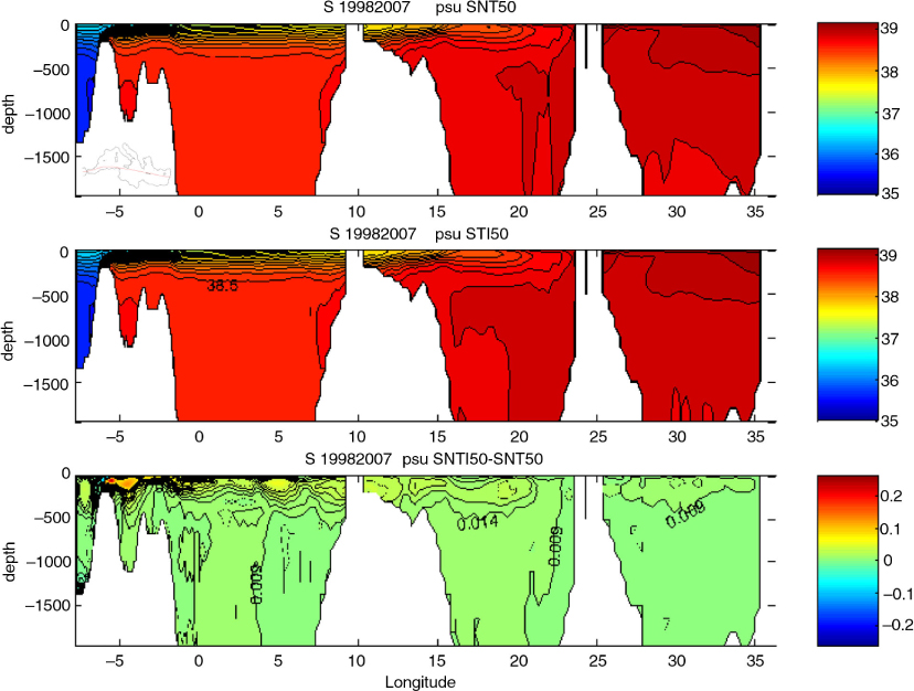
Fig. 16
As Fig. 15 but for salinity.