
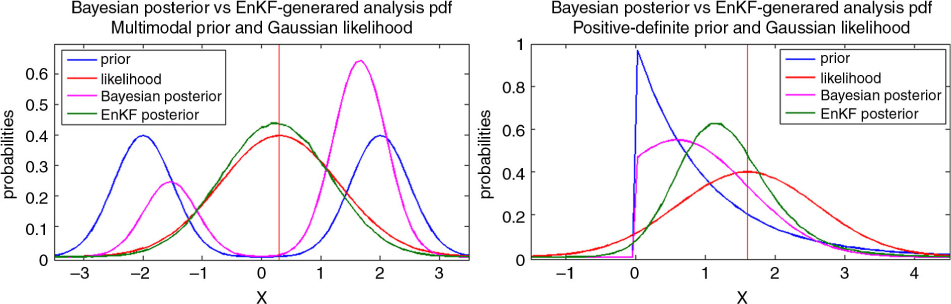
Fig. 1
Comparison of the analysis pdfs obtained by a direct application of the EnKF analysis step (green line) with respect to the actual Bayesian posteriors (magenta line). The state variables have either a multimodal prior distribution (left), or they are positive–definite quantities (right). The EnKF analysis step is applied with M=106.
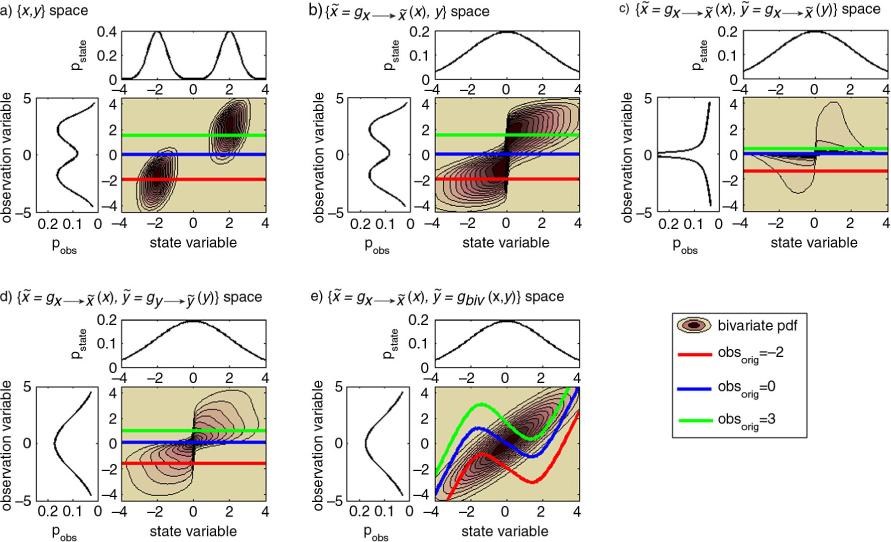
Fig. 2
Bivariate distributions (contour plots) and marginal distributions (line plots) for state variables (horizontal) and observations (vertical) under six different transformations [panels (a)–(e)] described in the text. Individual given observations are identified with colour lines in the contour plot, except for panel (f) where individual values of x are shown.
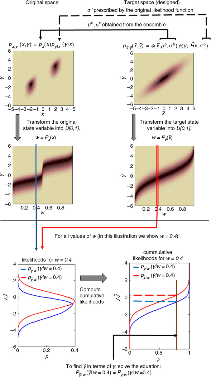
Fig. 3
The process for the joint state-space/observations transformation described in Section 4.2. First (i), a target probability space is constructed using the statistical moments inferred or prescribed by the original variables. Second (ii), the state variables (both original and transformed) are mapped into a random variable w distributed U[0,1]. Finally (iii), for each w an equation of cumulative likelihoods is solved to find y˜ in terms of y.
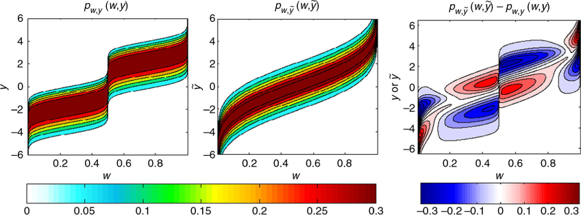
Fig. 4
Joint pdfs for the spaces {w, y} (left) and {w,[ytilde]} (centre). The difference between the two densities is plotted in the right panel.
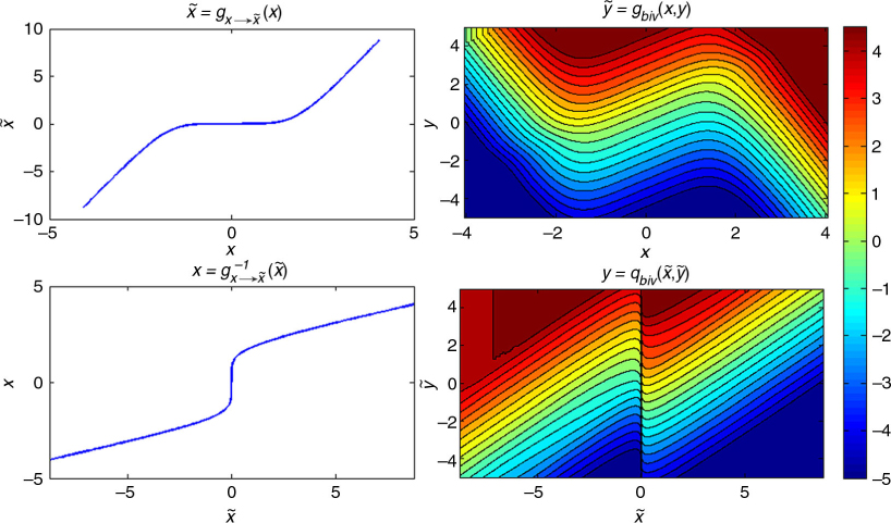
Fig. 5
Joint bivariate transformations from the {x,y} space (with GM marginals) to the space (with a joint bivariate Gaussian pdf). The first row shows the forward transformations: the state variable is univariately transformed (left) whereas the observation is transformed in a joint bivariately manner (right). The backward transformations are presented in the bottom row.
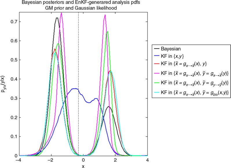
Fig. 6
Comparison of the Bayesian posterior distribution (black line) with respect to the EnKF-generated analysis pdfs, with the EnKF analysis step applied in five different spaces (colour lines) for a given observation (dotted vertical line). Both the prior and likelihood in the original space are GMs.
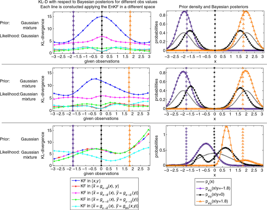
Fig. 7
Assessing the quality of the EnKF-generated analysis pdf's for three cases: GM–G (top row), GM–GM (centre row) and G–GM (bottom row). The left panels shows the D KL for the EnKF-generated analysis pdf's with respect to the Bayesian posterior (coloured lines) for different given observations (horizontal axis). In each case we choose three given observations (vertical lines with markers) and in the right panels we show the Bayesian posteriors associated with those three observations (coloured lines with markers, the colours correspond to those of the vertical lines). The solid grey curve in these panels represents the prior for each case.