
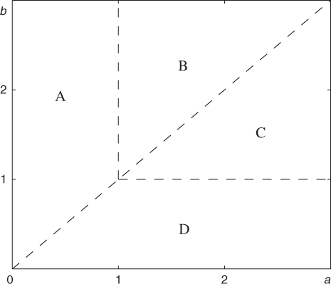
Fig. 1
Zones of equilibria.
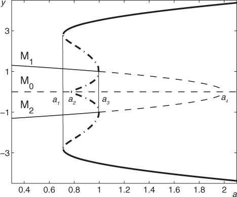
Fig. 2
Bifurcation diagram: y-coordinates of stable equilibria (thin solid lines), unstable equilibria (dashed lines), extrema of stable cycles (thick solid lines) and extrema of unstable cycles (dash-dotted lines).
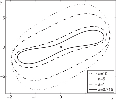
Fig. 3
Cycles of the deterministic system for b=2.
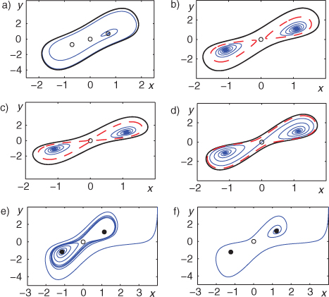
Fig. 4
Phase portraits of the deterministic system with b=2 for (a) a=1.5, (b) a=0.8, (c) a=0.76, (d) a=0.715, (e) a=0.7, (f) a=0.5 Stable cycles (thick solid black lines), unstable cycles (dashed red lines), stable equilibria (filled circles), unstable equilibria (empty circles) and phase trajectories (thin blue solid lines).
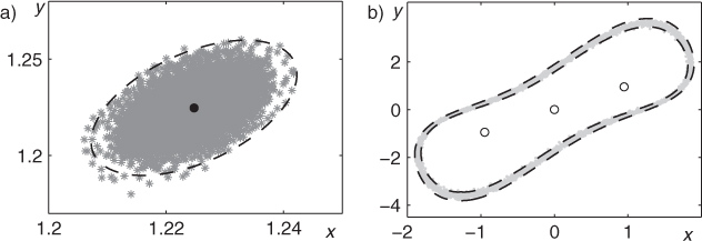
Fig. 5
Random states (grey) of stochastic attractors and confidence domains (dashed lines): (a) confidence ellipse around the equilibrium M 2 for a=0.5, ɛ=0.01; (b) confidence band around the limit cycle for a=1.1, ɛ=0.05.

Fig. 6
Stochastic sensitivity of attractors: (a) plots m(t) for cycles; (b) plots for equilibria and M(a) for cycles.
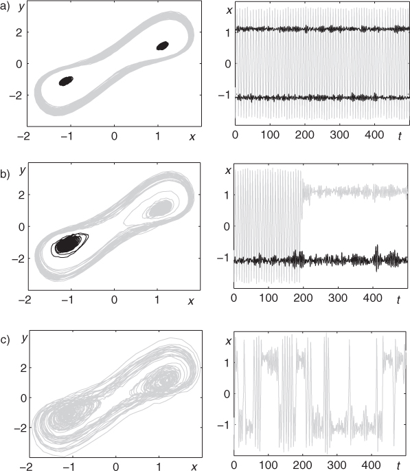
Fig. 7
Stochastic trajectories for a=0.76 and (a) ɛ=0.05; (b) ɛ=0.1; (c) ɛ=0.2.

Fig. 8
Stochastic trajectories for a=0.82 and (a) ɛ=0.05; (b) ɛ=0.1.

Fig. 9
Probability density function for ɛ=0.2 and (a) a=0.76; (b) a=0.82; (c) a=0.86.
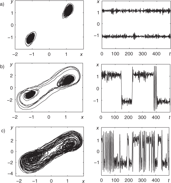
Fig. 10
Stochastic trajectories for a=0.7 and (a) ɛ=0.1; (b) ɛ=0.2; (c) ɛ=0.3.

Fig. 11
Plot of k(ɛ).
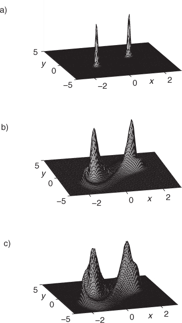
Fig. 12
Probability density function for a=0.7 and (a) ɛ=0.1; (b) ɛ=0.3; (c) ɛ=0.5.
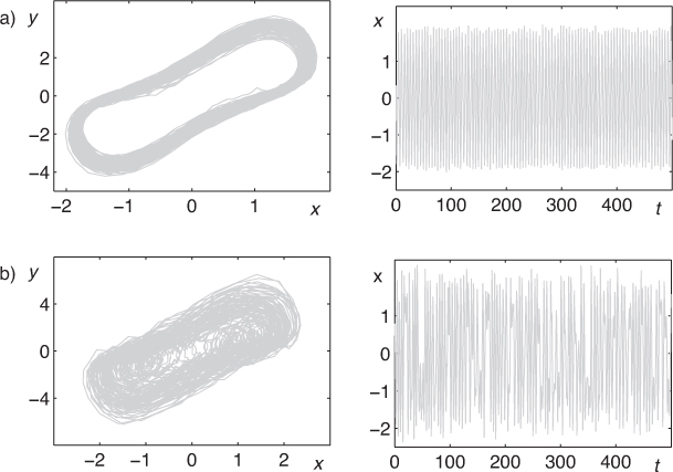
Fig. 13
Stochastic trajectories for a=1.1 and (a) ɛ=0.2; (b) ɛ=1.
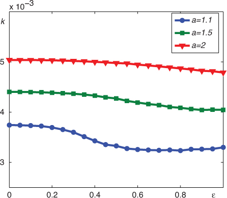
Fig. 14
Plot of k(ɛ).
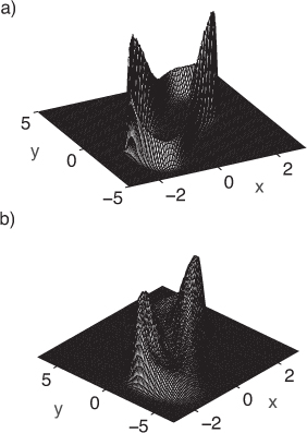
Fig. 15
Probability density function for a=1.1 and (a) ɛ=0.2; (b) ɛ=1.