
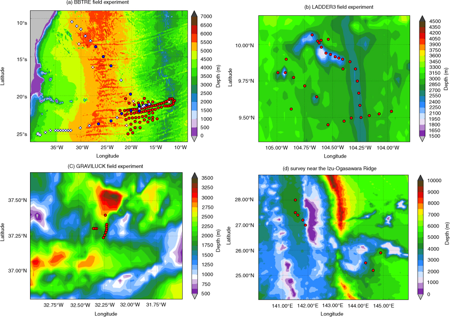
Fig. 1
(a) The locations of 75 stations during the BBTRE1 field experiment (blue circles) and those of 90 stations during the BBTRE2 field experiment (red circles). The cross-marked circles indicate the stations which are excluded in the analysis in this paper. (b) The locations of 37 stations during the LADDER3 field experiment. (c) The locations of 12 stations occupied in the GRAVILUCK field experiment. (d) The locations of 10 stations near the Izu-Ogasawara Ridge.
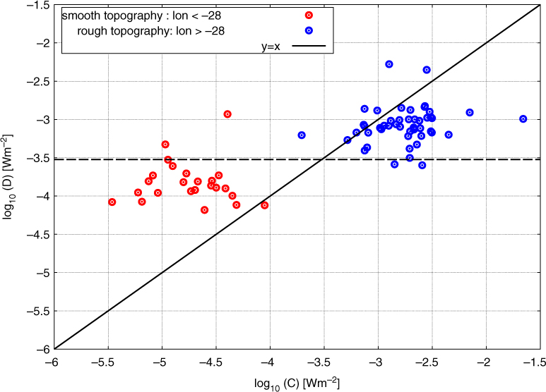
Fig. 2
Logarithmic scatter plot of the energy dissipation ɛ integrated up to 2000 m above the bottom, D, versus averages of the last 72 hours of vertical energy flux C=pw from model predictions. The weighted average of C at the observational sites is obtained from all the grid points within the radius γ. The diagram comprises 75 stations from the BBTRE1 survey, coloured according to the longitude of the observational site, so that the blue and red circles are the sites east and west of the longitude −28°, respectively.
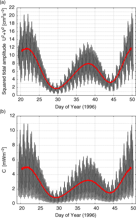
Fig. 3
(a) Time series of the squared barotropic-tide amplitude at station 64 from the BBTRE1 experiment in 1996. All the eight major tidal constituents have been taken into account to obtain the time series. (b) Time series of the energy flux C at this station when all the eight major tidal constituents have been taken into account. In both (a) and (b), the red solid lines show the 3-d running average of the time series.
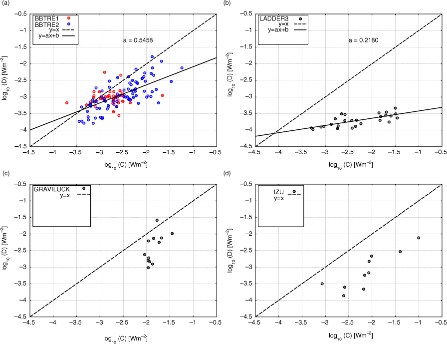
Fig. 4
(a) Logarithmic scatter plot of the energy dissipation rates ɛ integrated up to 2500 m above the ocean bottom versus the average of last 72 hours of the vertical energy flux C=pw for the 127 stations from the BBTRE1 and BBTRE2 experiments. The weighted average from all grid points within the radius γM 2 is used to obtain C at the observational sites. (b) As in (a), but for 26 stations from the LADDER3 experiment. The energy dissipation rates ɛ are integrated up to 1500 m above the bottom. (c) As in (a), but for 12 stations from the GRAVILUCK experiment. The energy dissipation rates are ɛ integrated up to 1500 m above the bottom. (d) As in (a), but for 10 stations near the Izu-Ogasawara Ridge (IZU dataset). The energy dissipation rates ɛ are integrated up to 2500 m above the ocean bottom.
Table 1. The optimal results of the statistical analysis carried out for BBTRE, LADDER3, GRAVILUCK and IZU datasets
BBTRE0.660.54580.00000.350.85LADDER30.710.21800.00490.020.20GRAVILUCK–––0.392.83IZU–––0.091.24
[i] The correlation coefficient r, the slope a of the fit line, and the p values are listed. Also shown are the ratio between the vertically integrated dissipation and the energy flux, d, when the optimal height above the ocean bottom is used to vertically integrate the energy dissipation, and the corresponding ratio d 10 when the energy dissipation is integrated vertically from the bottom to 10 m below the base of mixed layer. Note that d=0.05 for LADDER3 with correction for supercriticality.
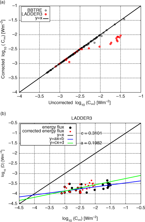
Fig. 5
(a) Logarithmic scatter plot of the corrected against the uncorrected values of the vertical energy flux C ∞ for 127 stations from the BBTRE experiment (black circles) and for 26 stations from the LADDER3 field survey (red circles). (b) Logarithmic scatter plot of the uncorrected C ∞ (black circles) and the corrected C ∞ (red circles) against the depth-integrated energy dissipation rate D for 26 stations from the LADDER3 field survey. The blue and green lines are the best-fit lines for the uncorrected C ∞ and the corrected C ∞, respectively.
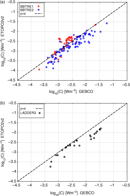
Fig. 6
(a) Logarithmic scatter plot of 72-hours averages of the energy flux C obtained using bathymetry data from GEBCO and from ETOPO2v2. The diagram comprises 127 stations from the BBTRE experiment. A weighted average over the grid points within the radius γM 2 is used to determine C at observational site. (b) As in (a), but for the 26 stations from the LADDER3 experiment.
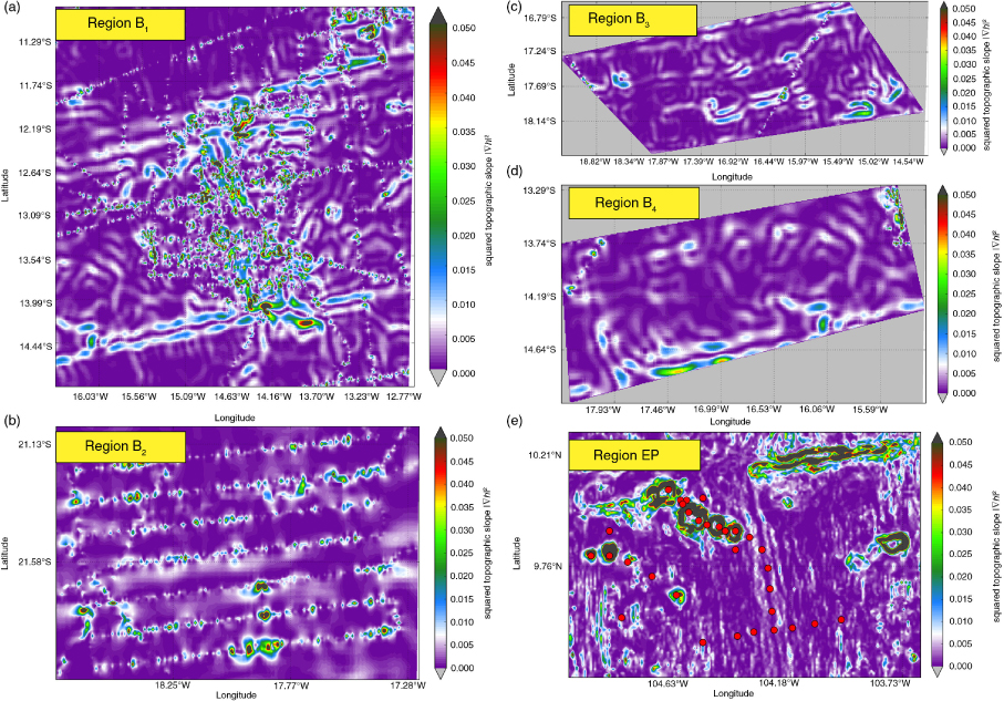
Fig. 7
(a) The squared bathymetry slope calculated from the GEBCO data for the region B1 with many ship tracks. (b) As in (a), but for the rectangular region B2 with many ship tracks. (c) As in (a), but for the region B3 with very few ship tracks. (d) As in (a), but for the region B4 with very few ship tracks. (e) As in (a), but for the region EP where the LADDER3 field survey was conducted. The red circles represent the 37 stations during this field survey. Note that there is approximately 50 km between two successive tick marks on the axes in Figs. (a)–(e).
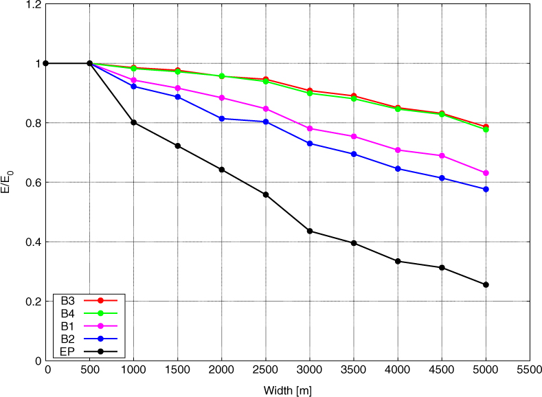
Fig. 8
The ratio E/E 0 against the width of the boxcar filter used to smooth the bathymetries of the five considered regions. E denotes the domain-integrated time-independent energy flux C ∞ associated with the M 2 tidal constituent, whereas E 0 denotes the value of E for the non-filtered bathymetry.
Table 2. Values of local dissipation efficiency q obtained in previous studies, and the regions for which q was defined
2002)0.3±0.1A large region above the Mid-Atlantic RidgePolzin (2004)1Entire Mid-Atlantic RidgeNiwa and Hibiya (2004)0.4East China Sea2006)0.35Hawaiian RidgeCarter et al. (2008)0.19Hawaiian RidgeZilberman et al. (2009)0.52A small subset of the Brazil BasinAlford et al. (2011)0.39Luzon Straits
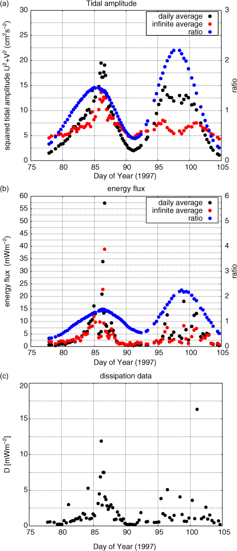
Fig. 9
(a) The average of the TPXO6.2-derived tidal flow amplitude squared U 2+V 2 over the last 24 hours of the time series prior to the measurement at each of 84 BBTRE2 stations (black dots), the infinite temporal average of U 2+V 2 at each of these stations (red dots), and the ratio between these two averages (blue dots). This ratio is multiplied by 10 for the better visualisation. (b) As in (a), but for the energy flux C. (c) the turbulent dissipations rates vertically integrated from the near-bottom up to 2500 m above the bottom for 84 BBTRE2 profiles. In all the panels, the horizontal axis pertains to ship-track time.
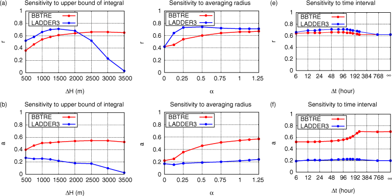
Fig. 10
(a) The correlation coefficient, r, between the energy flux log10(C Δt ) and the depth-integrated energy dissipation rate log10(D ΔH ) for various integration heights above the bottom ΔH. The weighted average from all the grid points located within the radius γM 2 is used to obtain the instantaneous vertical energy flux C at the observational points, which is then averaged over the last 72 hours of the time series, Δt=72 hours. (b) As in (a), but for the slope a of the fit line. (c) Correlation coefficient, r, for different averaging radii, αγM 2. Here, ΔH=2500 m for BBTRE and 1500 m for LADDER3, and Δt=72 hours. (d) As in (c), but for the slope a of the fit line. (e) The correlation coefficient for various time intervals Δt. ∞ on the horizontal axis corresponds to the long-term average of C, or C ∞. Here, ΔH=2500 m for BBTRE and 1500 m for LADDER3, and α = 1. (f) As in (e), but for the slope a of the fit line.