
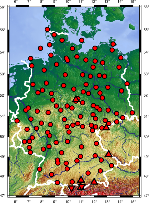
Fig. 1
Area of investigation and location of test sites. Triangles indicate mountain sites, diamonds indicate valley sites. Detailed information on test sites are presented in Supplementary file.

Fig. 2
Linear relationship of the distribution parameters In a and b for (a) wind speed and (b) gust speed based on hourly measurements. Mountain sites (green) and valley sites (cyan) are highlighted.
Table 1. Regression parameters of the relationship between distribution parameters In a and b for wind and gust speed dependent on the wind sector
WindGustWindGustWindGustWindGustRel. freq.17%20%27%36%
Correlation−0.79−0.80−0.88−0.91−0.75−0.79−0.90−0.93Slope−0.30−0.25−0.34−0.28−0.28−0.24−0.33−0.27Offset1.101.101.031.031.121.090.820.84
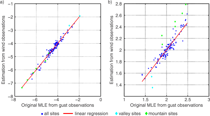
Fig. 3
Validation of the original against estimated distribution parameters for (a) scale parameter and (b) shape parameter. The original distribution parameters are based on the maximum-likelihood estimation (MLE) of the original dataset of gust measurements. The estimations are derived by the wind gust model using measurements of wind speed. Mountain sites are highlighted in green, valley sites in cyan.
Table 2. Validation of distribution parameters In a and b of measurements versus estimations dependent on the wind sector
ScaleCorrelation0.970.980.980.98Slope1.0011.0010.9990.999Offset0.0040.0020.000−0.002RMSE0.200.180.180.16ShapeCorrelation0.710.870.750.91Slope0.5990.8020.7030.948Offset0.7980.4200.6160.106RMSE0.160.140.160.10
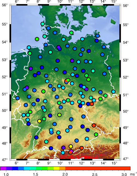
Fig. 4
RMSE of estimated gusts compared to measured gusts for the test sites.
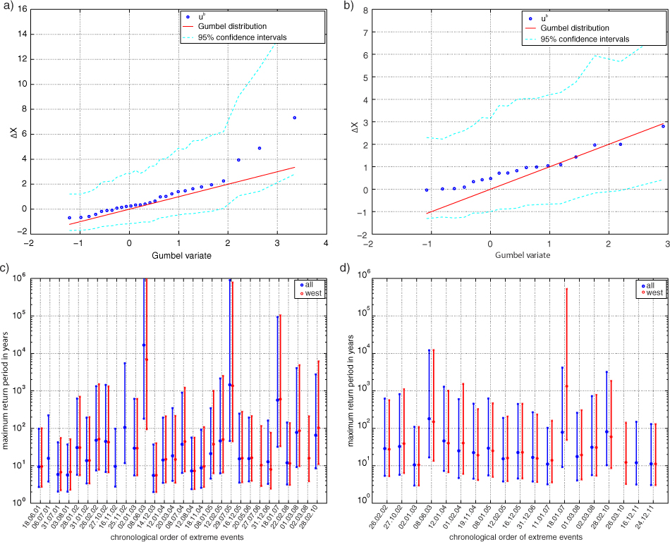
Fig. 5
Gumbel-plot for (a) measurements and (b) estimates and maximum return periods of locally strongest gusts identified in the dataset of (c) measurements and (d) estimations. The blue dots in the Gumbel plots (a, b) indicate ΔX n for independent extreme events based on all wind sectors, the red line shows the theoretical distribution, while the cyan lines show the 95% of the confidence intervals of ΔX n estimation. The blue dots in (c) and (d) indicate the return periods and their 95% confidence intervals for all wind sectors, while for red dots only the west sector was taken into account.
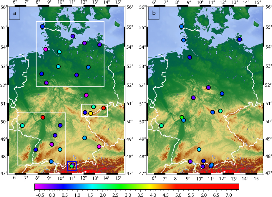
Fig. 6
Locations of occurrences of extreme gusts (maximum ΔX n ) for all directions for (a) measurements and (b) estimations from wind speeds. The white boxes mark the three main aggregations of extreme events shown in Fig. 5c. The blue box indicates the position of the two Foehn gusts.
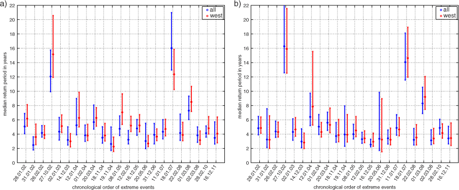
Fig. 7
Average return periods of extreme events in chronological order for (a) measurements and (b) estimations from wind speeds. Blue dots indicate the data basis of all directions, while red dots are based on the west sector only. Detailed estimates are presented in Table 3.
Table 3. Median return periods (Med. rp) of large-scale extreme events based on measurements and estimated gust values for all wind sectors. Events identified only from estimated gusts are marked with asterisks.
Anna26.02.20024.173.59–5.194.373.55–5.81Jennifer28.01.20025.074.06–6.884.833.90–6.47Lydia31.01.20022.471.79–3.623.242.12–7.55Jeanett27.10.200212.059.93–15.7416.2812.58–22.50Calvann02.01.20034.343.18–6.234.313.14–6.14Fritz14.12.20033.192.47–5.022.962.11–4.74Gerda12.01.20045.233.90–8.986.415.20–9.72Queenie*01.02.20043.842.99–5.275.053.95–6.74Oralie20.03.20045.684.71–8.065.604.53–7.06Pia18.11.20043.502.74–5.033.732.87–5.62Quimburga*19.11.20042.631.72–4.993.952.31–7.94Erwin08.01.20054.743.82–6.543.993.33–5.38Ulf12.02.20053.222.64–4.503.292.72–4.25Dorian16.12.20054.793.85–6.032.532.22–3.28Gertrud20.05.20063.031.97–5.523.351.72–9.82Karla31.12.20063.902.65–5.493.422.62–4.57Franz*11.01.20074.333.34–6.024.883.85–6.71Kyrill18.01.200716.0912.97–20.9814.0611.56–18.12Annette22.02.20084.163.13–6.793.202.49–4.79Emma01.03.20087.286.04–9.308.286.88–10.56Fee02.03.20083.832.85–5.003.122.53–4.60Xynthia28.02.20104.133.59–5.144.873.99–6.07Joachim*16.12.20113.472.61–5.723.402.64–5.09

Fig. 8
Spatial distribution of ΔX n during the storm Xynthia (28 Feb 2010) for (a) measured and (b) estimated gusts.

Fig. 9
Spatial distribution of ΔX n during the storm Kyrill (18 Jan 2007) for (a) measured and (b) estimated gusts.