
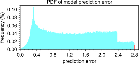
Fig. 1
The probability distribution function of prediction error when the model prediction time is set to 0.2 time units. The red bar represents the probability when the prediction errors are greater than 2.794000, while the maximum value of the prediction error of the exhaustive attack method is 2.794695.
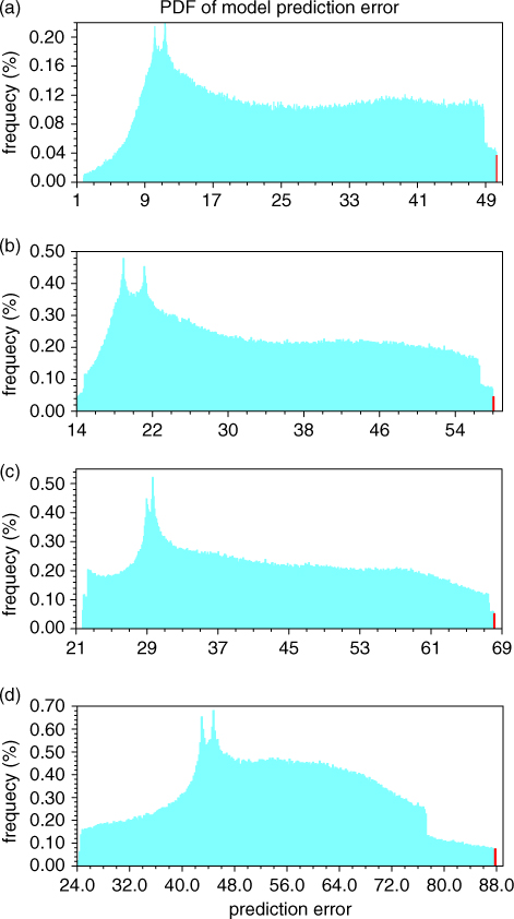
Fig. 2
Same as Fig. 1, except that the model prediction time is set to (a) 0.5, (b) 1.0, (c) 2.0 and (d) 3.0 time units. The red bar represents the probability when the prediction errors are greater than (a) 50.25, (b) 58.00, (c) 68.10 and (d) 87.70, respectively.
Table 1. CNOP-Ps with respect to an increasing model prediction time when the initial condition is fixed at (0.0, 1.0, 0.0)
0.550.29834(5.166220 E − 02, 8.557348 E − 02, −2.863084 E − 03)1.058.05844(−4.357523 E − 02, −8.960319 E − 02, 8.512808 E − 03)2.068.19016(−3.291568 E − 02, −9.348051 E − 02, 1.333990 E − 02)3.087.75441(−2.160796 E − 02, −9.635826 E − 02, 1.575380 E − 02)
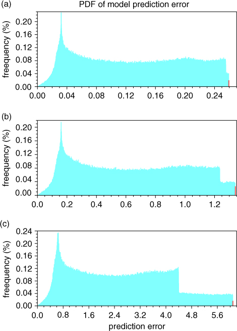
Fig. 3
Same as Fig. 1, except that the critical constraint value is set to (a) 0.01, (b) 0.05 and (c) 0.20. The red bar represents the probability when the prediction errors are greater than (a) 0.2594, (b) 1.3400 and (c) 6.0800, respectively.
Table 2. CNOP-Ps with respect to a varying critical constraint value when the prediction time is set to 0.2 time units and the model initial condition is fixed at (0.0, 1.0, 0.0)
0.013.420223 E − 020.2595067(5.920789 E − 03, 8.058799 E − 03, −4.983945 E − 06)0.050.17109821.340678(2.960444 E − 02, 4.029363 E − 02, −2.490810 E − 05)0.10.34241222.794697(5.921009 E − 02, 8.058637 E − 02, −4.911502 E − 05)0.20.68567516.082323(1.184327 E − 01, 1.611635 E − 01, −9.726922 E − 05)
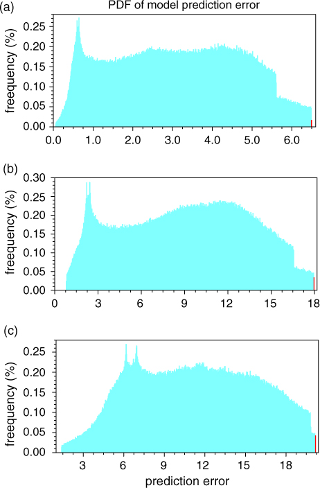
Fig. 4
Same as Fig. 1, except that the initial condition is set to (a) (1.0, 1.0, −1.0), (b) (5.0, 5.0, 5.0) and (c) (−10.0, −10.0, −10.0). The red bar represents the probability when the prediction errors are greater than (a) 6.49, (b) 17.95 and (c) 20.17, respectively.
Table 3. CNOP-Ps with respect to different initial conditions when the prediction time is set to 0.2 time units
(1.0, 1.0, −1.0)6.493985(3.640889 E − 02, 9.313641 E − 02, −5.553383 E − 05)(5.0, 5.0, 5.0)17.96980(2.122251 E − 02, 9.770686 E − 02, −1.724857 E − 03)(−10.0, −10.0, −10.0)20.19837(2.615064 E − 02, 9.611105 E − 02, −8.877495 E − 03)
Table 4. Optimised parameter values and corresponding optimised prediction errors with the prediction time set to 2.0 time units when random errors of different variances are added to the observations
0.013.258717(11.59596, 31.88207, 2.862262)130.044.851858(11.59111, 31.74486, 2.867236)130.097.159717(11.57233, 31.63118, 2.867709)13
Table 5. Optimised parameter values and corresponding optimised cost functions with the prediction time set to 0.2 time units and the critical constraint δ set to 0.30
(σ, r)2.698106 E − 04(11.49159, 32.01515, 8/3)9(σ, b)3.031157 E + 00(13.00000, 28, 2.665819)1(r, b)5.351562 E − 01(10, 23.85923, 3.362714)18(σ, r, b)2.717061 E − 04(11.49203, 32.01417, 2.666177)10
Table 6. Local CNOP-Ps with respect to an increasing model prediction time when the model initial condition is fixed at (0.0, 1.0, 0.0)
0.548.77164(−5.727754 E − 02, −8.192971 E − 02, 2.608925 E − 03)1.056.57906(4.356946 E − 02, 8.968048 E − 02, −7.688598 E − 03)2.067.49694(3.075451 E − 02, 9.356575 E − 02, −1.730929 E − 02)3.077.14283(1.979255 E − 02, 9.762610 E − 02, −8.797674 E − 03)