
Table 1. Notations for variables and constants in prognostic equations (1)–(8)
tTimerRadiuszHeightuRadial velocityvTangential velocitywVertical velocityVHorizontal wind speedΠNon-dimensional pressure (Exner function)ρAir densityTAbsolute temperatureθPotential temperatureq v Mass fraction of water vapourq c Mass fraction of cloud waterq r Mass fraction of rain waterJ G Vertical diffusive mass flux of substance G(G=dry air, water vapour, cloud water, rain water)ΦDissipation rateQ R Radiative heating rateD ρG Micro-turbulent flux of quantity G(G=u,v,w,θ,q v ,q c ,q r )c p Specific heat capacity of air at constant pressurec pd 1005 Jkg−1K−1Spec. heat capacity of dry airc pv 1848 Jkg−1K−1Spec. heat capacity of water vapourc pl 4185 Jkg−1K−1Spec. heat capacity of liquid waterR d 287.0 Jkg−1K−1Spec. gas constant of dry airR v 461.5 Jkg−1K−1Spec. gas constant of water vapourl v 2.5·10−6Jkg−1Latent heat of vapourisationf5·10−5s−1Coriolis parameterg9.81 ms−2Gravitational acceleration
Table 2. Characteristics of different experimental set-ups in HURMOD
Case INon-neutralTime-invariant tropopause temperature T t Case JNon-neutralTime-invariant tropospheric lapse rate ΓCase NMoist-neutral
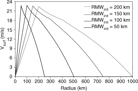
Fig. 1
Initial tangential surface velocity as a function of radial distance to the centre for four different values in the initial RMW (50 km, 100 km, 150 km, 200 km).
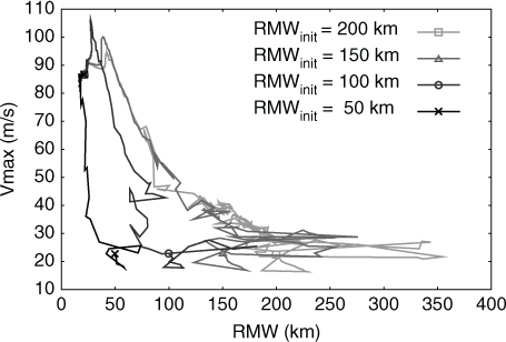
Fig. 2
Trajectories in a phase diagram spanned by maximum horizontal wind speed and RMW for different initial RMW values (50 km, 100 km, 150 km, 200 km). A marker is plotted at the starting point (t=0 h) and the final point (t=4000 h) on each trajectory.
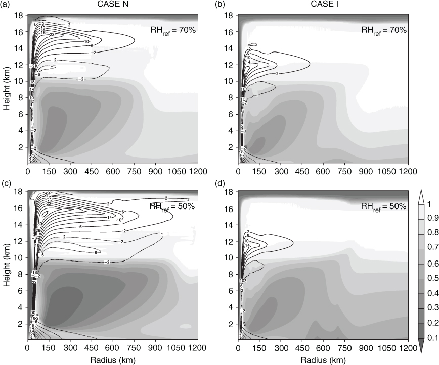
Fig. 3
Radial velocity (contour lines) and relative humidity (shadings) fields for two different values in initial tropospheric relative humidity: RH ref =70% in the upper panels (a) and (b), and RH ref =50% in the lower panels (c) and (d). Stable state results averaged over the last 120 h for case N are displayed on the left, and those for case I on the right.
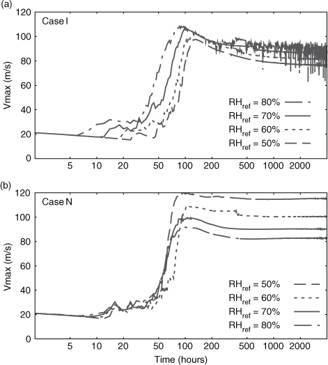
Fig. 4
Time development of maximum horizontal wind speed for (a) case I with a constant equilibrium tropopause temperature of T s=−70°C and (b) the moist-neutral case N, in simulations with differing parameter values for the reference relative humidity, RH ref . Note: The time scale is logarithmic.
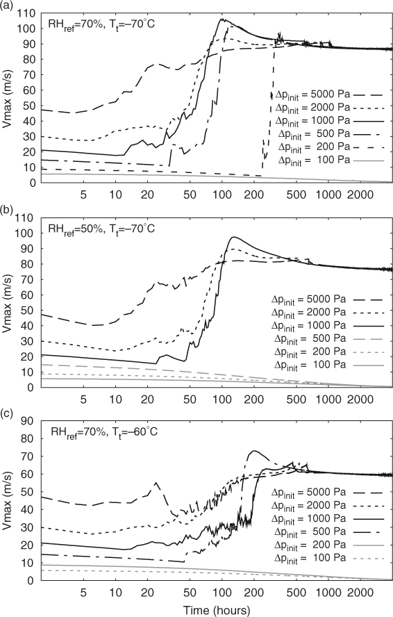
Fig. 5
Time development of maximum horizontal wind speed in case I, for varying initial vortex strength given by the initial central surface pressure difference, Δp init , between the core and the environment in simulations with differing parameter values for the reference relative humidity, RH ref , and the tropopause temperature, T t , from top to bottom: (a) RH ref =70% and T t =−70°C, (b) RH ref =50% and T t =−70°C, and (c) RH ref =70% and T t =−60°C. Initial disturbances that reach TC strength are displayed by black lines, non-developing systems by grey lines.
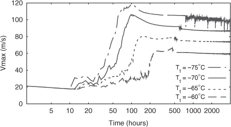
Fig. 6
Time development of maximum horizontal wind speed for case I in simulations with differing parameter values for the tropopause temperature, T t .
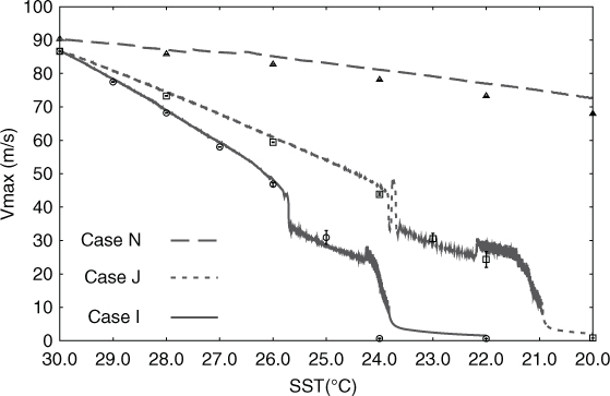
Fig. 7
Development of maximum horizontal wind speed with decreasing SST with time at a cooling rate of 10−3°C/h for the moist-neutral case N (dashed line), case J with Γ=const (dotted line) and case I with T t =const (solid line). Average values over the last 120 h of the 4000 h-runs at fixed SSTs are plotted with different markers for case N (triangles), case J (squares) and case I (circles). Error bars display the full range of maximum wind speed during the last 120 h of the long-term runs.
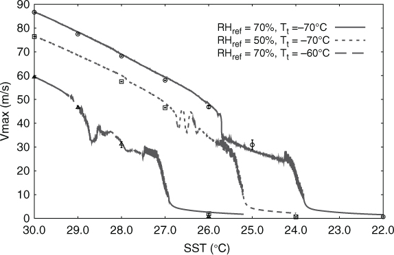
Fig. 8
Development of maximum horizontal wind speed with decreasing SST with time at a cooling rate of 10−3°C/h in case I for three simulations with differing parameter values for the reference relative humidity, RH ref , and the tropopause temperature, T t . Average values over the last 120 h of the 4000 h-runs at fixed SSTs are plotted with different markers for RH ref =70% and T t =−70°C (circles), RH ref =50% and T t =−70°C (squares), and RH ref =70% and T t =−60°C (triangles). Error bars display the full range of maximum wind speed during the last 120 h of the long-term runs.
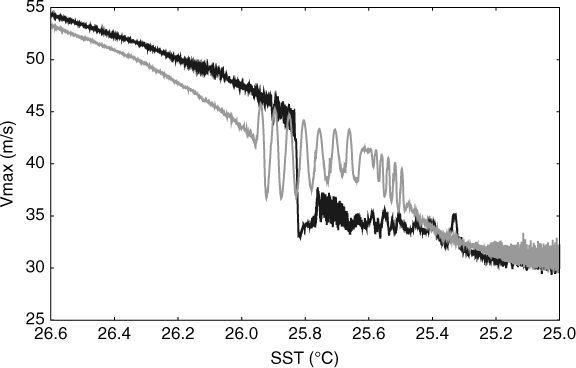
Fig. 9
Development of maximum horizontal wind speed with decreasing SST (dark grey line) and increasing SST (brighter grey line) in time at a rate of 2·10−4°C/h.
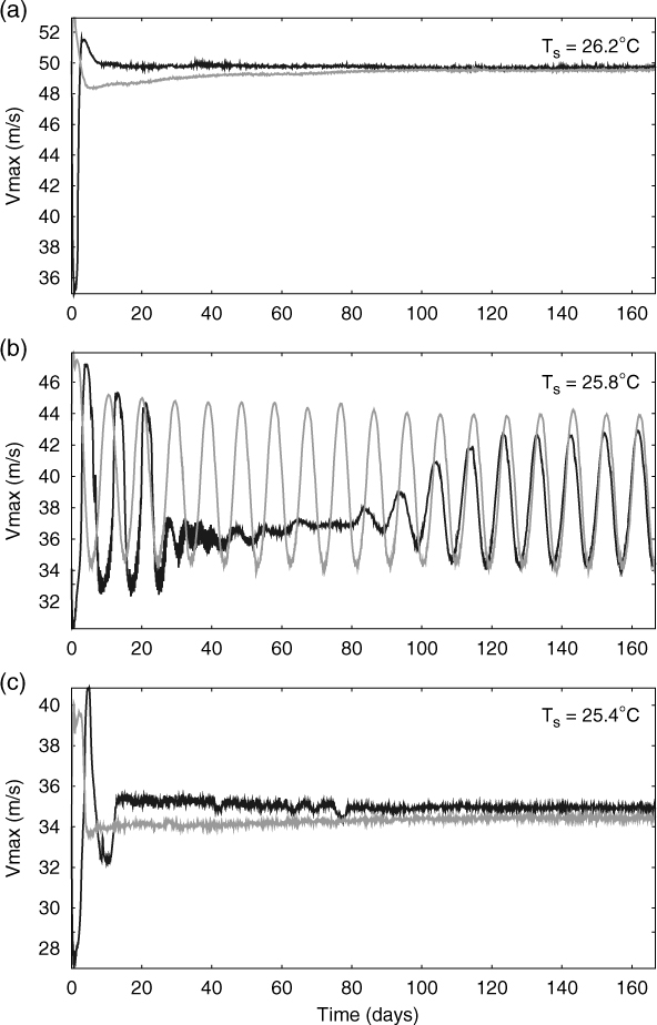
Fig. 10
Time development of maximum horizontal wind speed in case I for fix SST values in the vicinity of the bifurcation from top to bottom: (a) T s=26.2°C, (b) T s=25.8°C and (c) T s=25.4°C. Each simulation was started at the respective SST from the simulation with decreasing SST (dark grey lines) and increasing SST (brighter grey line) in time (cf. Fig. 9).
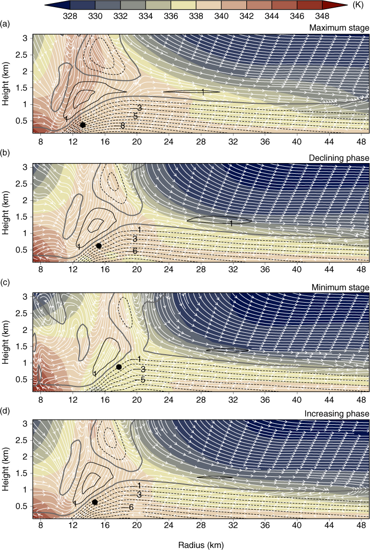
Fig. 11
Equivalent potential temperature θ e (colour shadings), stream lines (white) and radial velocity (contour lines) at lower tropospheric levels for the inner part of the TC in the case I standard configuration at different phases of the limit cycle from top to bottom: (a) maximal intensity at maximum, (b) declining intensity, (c) minimal intensity and (d) increasing intensity. Higher θ e -values are displayed in reddish shades, lower θ e -values in bluish shades. Inward flow is indicated by dashed lines, zero-radial velocity by thick grey line and outward flow by solid black lines. The contour interval is 1 m/s. The location of V max is marked by a black circle.
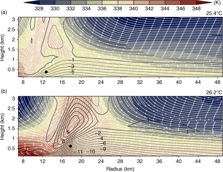
Fig. 12
As in Fig. 11, but for the respective stable states surrounding the limit cycle: (a) at T s=25.4°C and (b) T s=26.2°C.
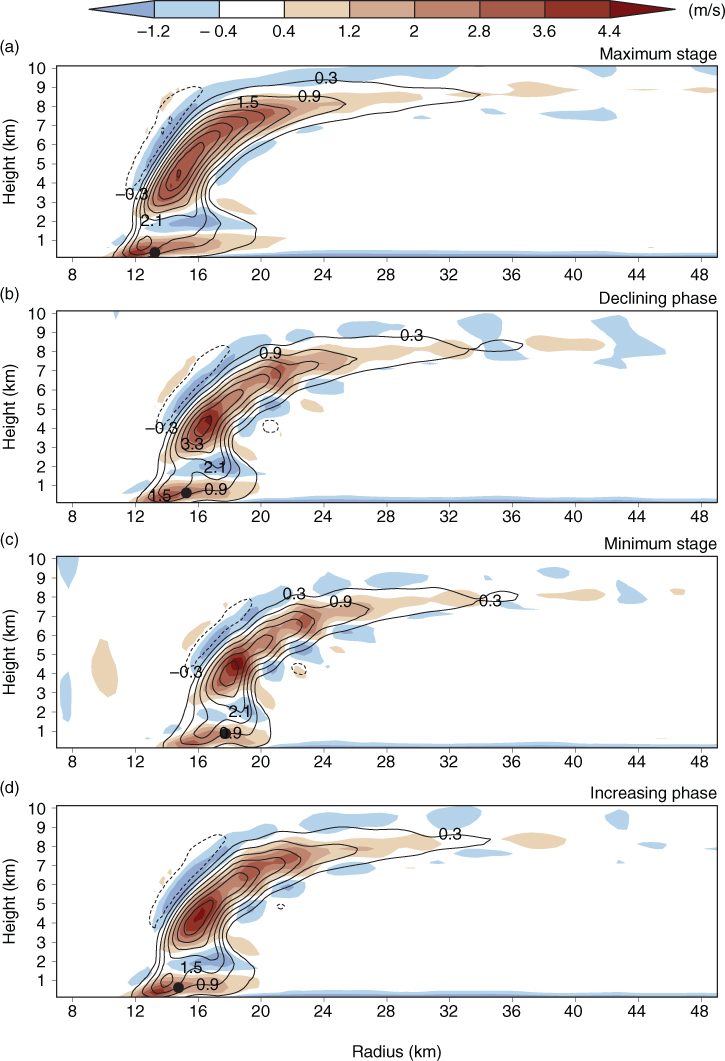
Fig. 13
Difference between tangential wind and gradient wind (colour shadings), and vertical velocity (contour lines) for the inner part of the TC in the case I standard configuration at different phases of the limit cycle from top to bottom: (a) maximal vortex strength, (b) declining strength, (c) minimal strength and (d) increasing strength. Red shades indicate supergradient winds, blue shades indicate subgradient winds, and white areas are in or close to gradient wind balance. Downward flow is indicated by dashed lines and upward flow by solid lines. The contour interval is 0.6 m/s. The location of V max is marked by a black circle.
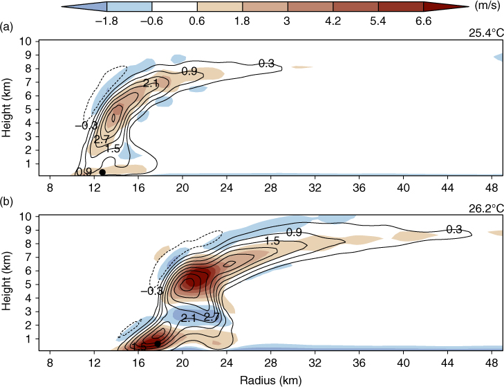
Fig. 14
As in Fig. 13, but for the respective stable states surrounding the limit cycle: (a) at T s=25.4°C and (b) T s=26.2°C. Note: The colour scale interval is larger than in Fig. 13.
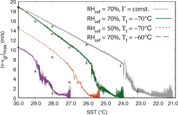
Fig. 15
Development of maximum supergradient wind, (v–v gr ) max , with decreasing SST with time at a cooling rate of 10−3°C/hin the standard configuration of case J (grey solid line), and case I with differing parameter values: RH ref =70% and T s=−70°C (green solid line), RH ref =50% and T s=−70°C (orange dotted line), and RH ref =70% and T t =−60°C (purple dashed line). Average values over the last 120 h of the 4000 h-runs at fixed SSTs are plotted with different markers for case J (diamonds), case I with RH ref =70% and T t =−70°C (circles), RH ref =50% and T t =−70°C (squares), and RH ref =70% and T t =−60°C (triangles). Error bars display the full range of maximum supergradient wind during the last 120 h of the long-term runs.
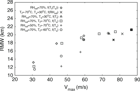
Fig. 16
Radius of maximum wind speed (km) versus maximum horizontal wind speed (m/s) from average values over the last 120 h of the 4000 h-runs at different values for T s and T t =f(T s) in case J (diamonds), and case I with T t =−70°C and T t =30°C for different values in RH ref (crosses), RH ref =70% and T s=30°C for different values in T t (triangles), RH ref =70% and T t =−70°C for different values in T s (squares), RH ref =50% and T t =−70°C for different values in T s (plus signs), and RH ref =70% and T t =−60°C for different values in T s (circles). Note: identical results in this plot stem from the same model experiment.
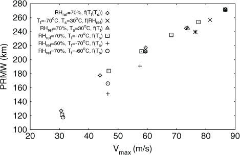
Fig. 17
As in Fig. 16, but with the potential radius of maximum wind speed on the ordinate.