

Fig. 1
Initial conditions and their evolutions with the linear advection–diffusion equation: (a) flat top-hat (FTH), (b) quadratic top-hat (QTH), (c) window sinusoid (WS), and (d) squared-exponential (SE). The first two initial conditions (a, b) exhibit sparse representation in the wavelet domain while the next two (c, d) show nearly sparse representation in the discrete cosine domain (DCT). Initial conditions are evolved under the linear advection–diffusion eq. (15) with and a=1[L/T]. The broken lines show the time instants where the low-resolution and noisy observations are available in the assimilation interval.
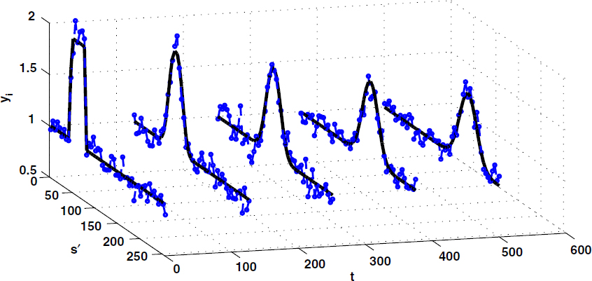
Fig. 2
A sample representation of the available low-resolution (solid lines) and noisy observations (broken lines with circles) in every 125 [T] time-steps in the assimilation window for the flat top-hat (FTH) initial condition. Here, the observation error covariance is set to with σ r =0.08 equivalent to .
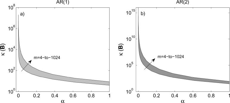
Fig. 3
Empirical condition numbers of the background error covariance matrices as a function of parameter α and problem dimension (m) for the AR(1) in (a) and AR(2) in (b). The parameter α varies along the x-axis and m varies along the different curves of the condition numbers with values between 4 and 1024. We recall that is the ratio between the largest and smallest singular values of B. In (a) the covariance matrix is and in (b) , . It is seen that the condition numbers of the AR(2) model are significantly larger than those of the AR(1) model for the same values of the parameter α.
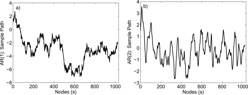
Fig. 4
Sample paths of the used correlated background error: (a) the sample path for the AR(1) covariance matrix with α −1=150, and (b) the sample path for the AR(2) covariance matrix with α −1=25. The paths are generated by multiplying a standard white Gaussian noise from the left by the lower triangular matrix L, obtained by Cholesky factorisation of the background error covariance matrix, that is B=LL T. It is seen that for small α, the sample paths exhibit large-scale oscillatory behaviour that can potentially corrupt low-frequency components of the underlying state.
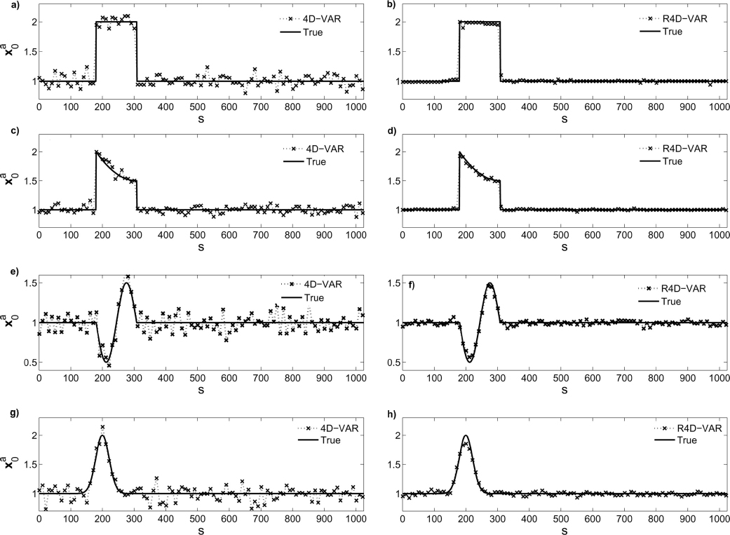
Fig. 5
The results of the classic 4D-Var (left panel) versus the results of -norm R4D-Var (right panel) for the tested initial conditions in a white Gaussian error environment. The solid lines are the true initial conditions and the crosses represent the recovered initial states or the analysis. In general, the results of the classic 4D-Var suffer from overfitting while the background and observation errors are suppressed and the sharp transitions and peaks are effectively recovered in the regularised analysis.
Table 1. Expected values of the MSE r , MAE r , and BIAS r , defined in eq. (20), for 30 independent runs
MSE r MAE r BIAS r
R4D-Var4D-VarR4D-Var4D-VarR4D-Var4D-Var
FTH0.01880.06900.00990.05890.00160.0004QTH0.01520.05150.00830.04140.00300.0016WS0.02960.09590.02290.07710.00380.0022SE0.03160.08990.02350.07280.00184.26 e–5
[i] The background and observation errors are white (, ), where σ b =0.10 (dB) and σ r =0.08 (dB). The initial conditions are: flat top-hat (FTH), quadratic top-hat (QTH), window sinusoid (WS), and squared-exponential (SE). The results are reported for both the classic 4D-Var and the regularised 4D-Var (R4D-Var).
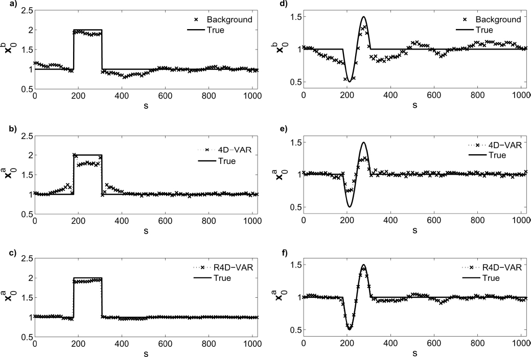
Fig. 6
Comparison of the results of the classic 4D-Var (b, ; e) and -norm R4D-Var (c, ; f) for the top-hat (left panel) and window sinusoid (right panel) initial conditions. The background states in (a) and (d) are defined by adding correlated errors using an AR(1) covariance model of , where α=1/250. The results show that the -norm R4D-Var improves recovery of sharp jumps and peaks and results in a more stable solution compared to the classic 4D-Var; see Fig. 7 for quantitative results.
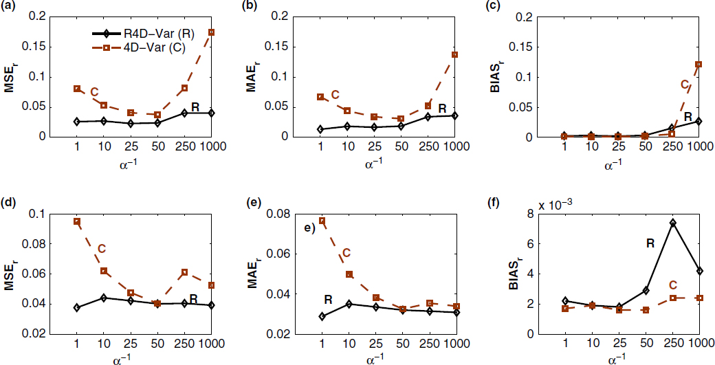
Fig. 7
Comparison of the results of the proposed -norm R4D-Var (solid lines) and the classic 4D-Var (broken lines) under the AR(1) background error for different correlation characteristic length scales (α −1). Top panel: (a–c) the chosen quality metrics for the top-hat initial condition (FTH); Bottom panel: (d–f) the metrics for the window sinusoid initial condition (WS). These results, averaged over 30 independent runs, demonstrate significant improvements in recovering the analysis state by the proposed -norm R4D-Var compared to the classic 4D-Var.
Table 2. Expected values of the MSE r , MAE r , and BIAS r , defined in (20), for 30 independent runs
MSE r MAE r BIAS r
α−1R4D-Var4D-VarR4D-Var4D-VarR4D-Var4D-Var
FTH10.02540.07540.01620.06290.00230.001650.03280.06430.02120.05340.00430.0018250.0722–0.0608–0.0187–500.0742–0.0582–0.0268–WS10.03630.08870.02720.07150.00290.001250.07080.09060.05710.05290.01060.0017250.0877–0.0710–0.0243–500.0898–0.0747–0.0361–
[i] The background and observation errors are modelled by the first order auto-regressive () and white () Gaussian processes, where σ b =0.10 (dB) and σ r =0.08 (dB). The parameter α denotes the correlation decay rate in the AR(2) covariance function . The studied initial conditions are: flat top-hat (FTH), and window sinusoid (WS) and the results are reported for both the classic 4D-Var and the regularised 4D-Var (R4D-Var). The dash lines in the table denote that the classic method failed to return a solution without any pre-conditioning.
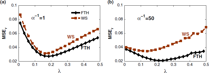
Fig. 8
The relative mean squared error versus the regularisation parameter obtained for the AR(1) background error for different characteristic correlation length (a) α −1=1, and (b) α −1=50. FTH and WS denote the flat top-hat (FTH) and window sinusoid initial conditions, respectively.