
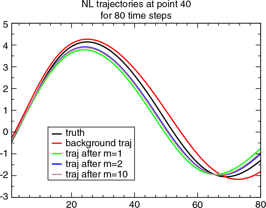
Fig. 1
Time series of L96-values at point j=40. Time t 0=0dt corresponds to the start of the assimilation window; the end of the assimilation window is at t 1=20dt; the final forecast range displayed is at t f =80dt. The time unit is in model iterations. The black, red and brown curves, respectively, represent the trajectories computed from the truth, the background and the analysis states for run 1 out of the 10 random realizations when σ o =σ b =0.2. The green and blue curves show trajectories obtained during the non-linear minimization process for m=1,2, resp.
Table 1. Values of the various sensitivity diagnostics evaluated at verification times t v =40dt=0.4 and t v =80dt=0.8 for the case when σ o =σ b =0.2. Incremental estimates for midpoint, Simpson, , and are given for m=10, and thus also correspond to the values for m=10, t v =0.8 in Figure 2. The values are for one given occurrence out of the 10 random realizations (run 1). The mean relative error is with respect to the true reduction and averaged over all occurrences. It is given in percentages.
δet v =0.4t v =0.4t v =0.8t v =0.8δe1−6.96177.55−20.88105.59δe2−2.586.27−11.4010.64δe LB −2.524.50−8.058.17δe mid −2.574.18−10.533.67δe Simp −2.562.05−9.701.73−2.604.43−12.036.84−2.561.98−9.801.77−10.57253.01−33.68170.59−2.7811.93−14.9123.93−2.511.65−9.2721.95Truth−2.64—−10.67—
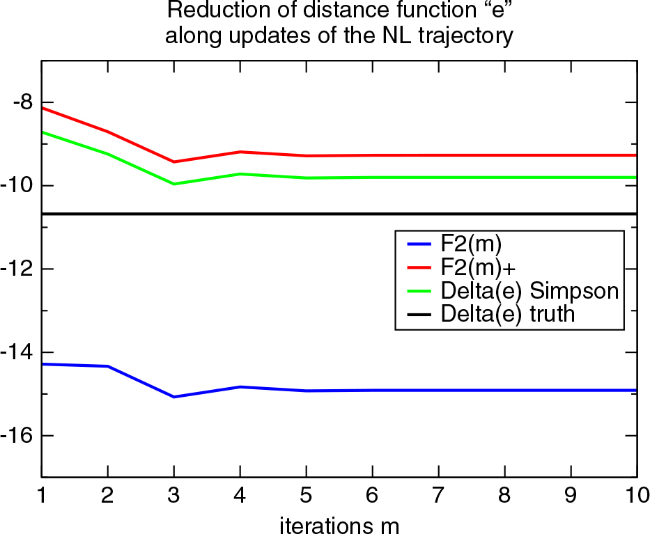
Fig. 2
Successive values of the cumulative variations , and DT09's Simpson rule quadrature estimate, for the 10 successive loops m=1,10 when σ o =σ b =0.2 (blue, red, green, resp.). The curves are for run 1 of the 10 random occurrences of the assimilation problem. Verification time is t v =80dt=0.8.