
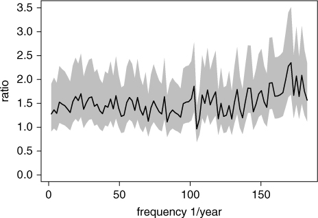
Fig. 1
Exemplary ratio of the RCM spectrum and the GCM spectrum for one grid cell in the Pacific (140°E, 20°N) for T850 in winter taken from the ‘20C’ experiment. The shaded area indicates the 95% confidence interval.
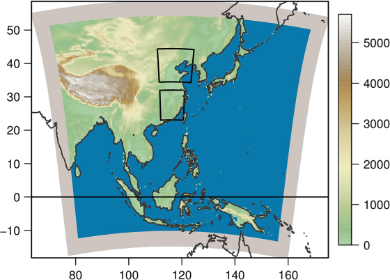
Fig. 2
Orography [m a.m.s.l.] for the East Asia domain in 0,44°resolution. The grey frame indicates the sponge zone. Two subdomains (North—Haihe, South—Poyang) are highlighted by boxes.
Table 1. Simulations performed with COSMO-CLM for East Asia
ModelCOSMO_4.8_CLM_11 (and higher)
Horizontal resolution0,44° (50 km)0,0625° (7 km)
Horizontal grid size (excl. sponge zone)183×147160×160128×144Timestep150s60s
Convection schemeTiedtke
Time interval for boundary conditions6 hours
Driving model & simulated periodERA40 1971–2000 (CCLM_eval_50km)CCLM_eval_50km 1971–2000CCLM_eval_50km 1971–1975ECHAM5_20C3M_all_3 1971–2000 (CCLM_20C_50km)CCLM_20C_50km 1971–2000CCLM_20C_50km 1971–1997ECHAM5_A1B_3 2011–2050 (CCLM_A1B_50km)CCLM_A1B_50km 2021–2050CCLM_A1B_50km 2021–2050
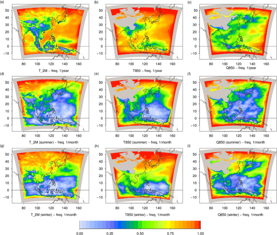
Fig. 3
Grid-point wise coherence between COSMO-CLM (0,44°resolution) driven by ECHAM5 20C3M_all run no.3 and ECHAM5 20C3M_all run no.3. The 1st, 2nd and 3rd columns show results for the variables T_2M, T850 and Q850, respectively. The 1st, 2nd and 3rd rows show results for the frequencies 1/yr, 1/month in summer and 1/month in winter, respectively. The grey frame indicates the sponge zone. The grey shaded areas within the domain cover mountainous regions, that lie above 850 hPa.
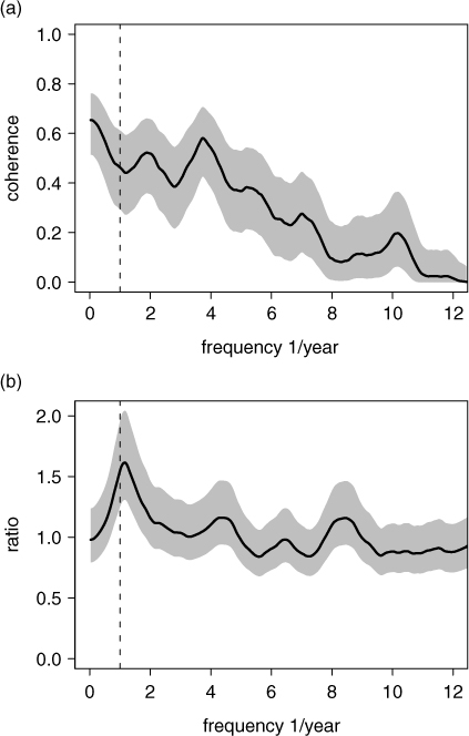
Fig. 4
Analysis of T_2M averaged over the box 4°N to 9°N and 132°E to 144°E. (a) Coherence between the time series from COSMO-CLM driven by ECHAM5 20C3M_all run no.3 and ECHAM5 20C3M_all run no.3. (b) The ratio between the corresponding univariate spectra.
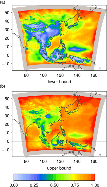
Fig. 5
95% confidence interval for T_2M at the frequency 1/yr (Fig. 3a).
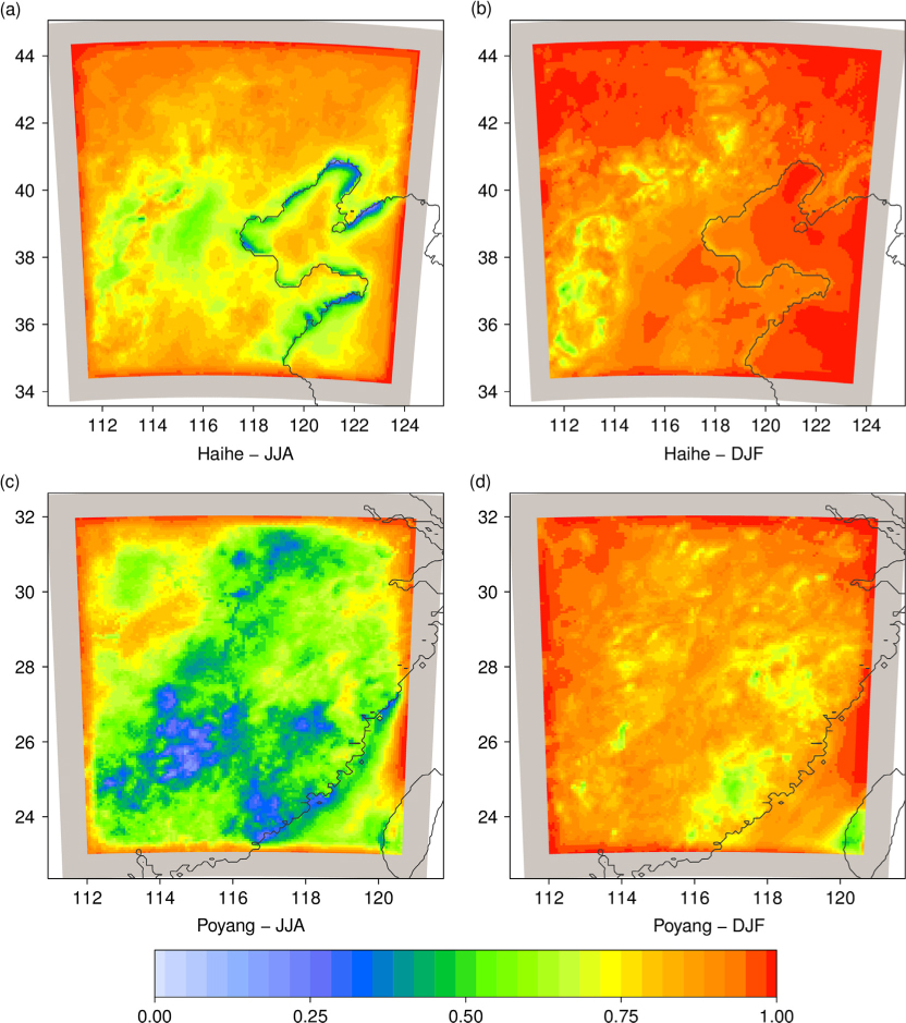
Fig. 6
Grid-point wise coherence at frequency 1/48h between COSMO-CLM (0,0625°resolution) driven by COSMO-CLM ‘20C’ (0,44°resolution) and COSMO-CLM ‘20C’ (0,44°resolution). The 1st and 2nd columns show the results for COSMO-CLM (0,0625°) adapted to the Haihe catchment and the Poyang catchment, respectively. The 1st and 2nd rows show the results for summer season (JJA) and winter season (DJF), respectively. The grey frame indicates the sponge zone.
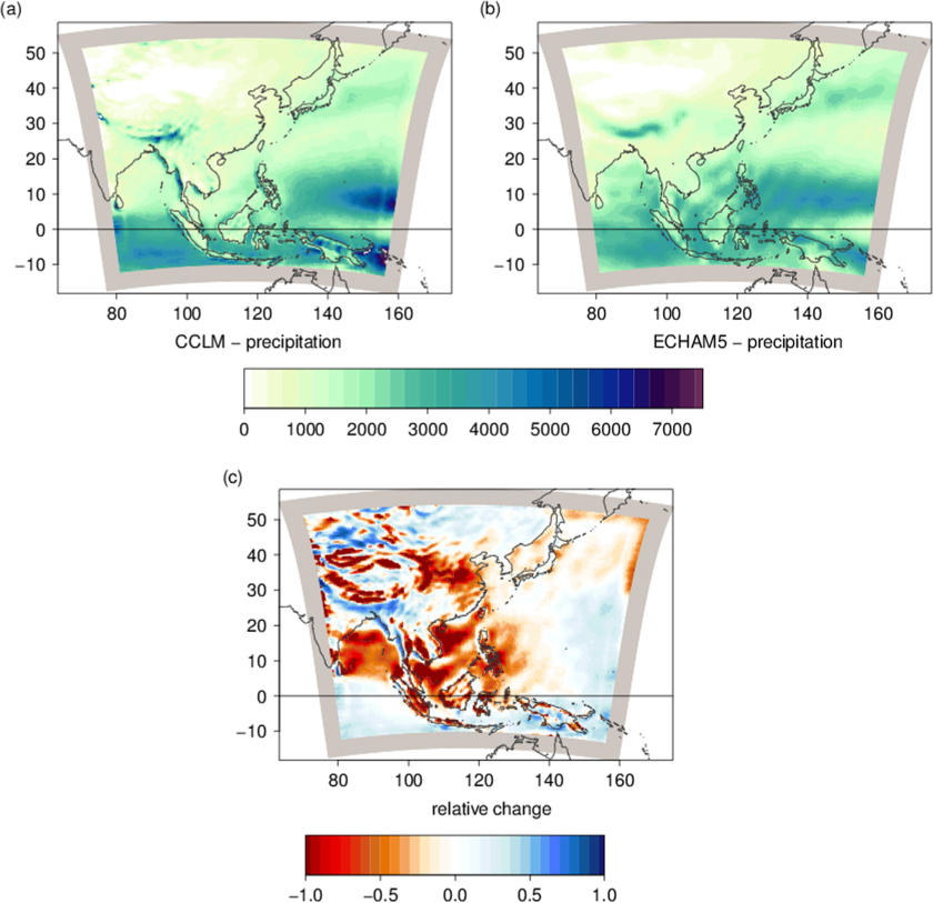
Fig. 7
Comparison of mean annual precipitation from COSMO-CLM and ECHAM5 for the period from 1971 to 2000 in mm. The field of ECHAM5 is bi-linearly interpolated to the COSMO-CLM grid and the sponge frame is added for better visual orientation. The right-hand plot shows the relative change between COSMO-CLM values and ECHAM5 values, with the darkest red indicating a relative change of –100% or less.
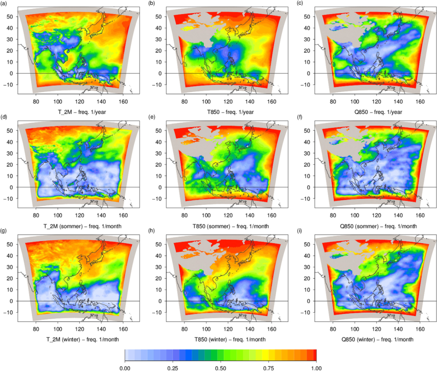
Fig. 8
Grid-point wise coherence between COSMO-CLM (0,44 °resolution) driven by ERA-40 and ERA-40. The 1st, 2nd and 3rd columns show results for the variables T_2M, T850 and Q850, respectively. The 1st, 2nd and 3rd rows show results for the frequencies 1/yr, 1/month in summer and 1/month in winter, respectively. The grey frame indicates the sponge zone. The grey shaded areas within the domain cover the mountainous regions that lie above 850 hPa and contain only artificial results for T850 and Q850.
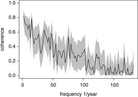
Fig. 9
A exemplary coherence spectrum for one grid cell in the Pacific (140°E, 20°N) for T850 in winter taken from the ‘20C’ experiment. The grey shaded area indicates the 95% confidence interval.