
1. Introduction
Forecast skill in numerical weather prediction is affected by two types of error: initial condition error and model error. The magnitudes of model error and initial condition error have changed over the decades as forecast models, data assimilation and the global observing network have become more sophisticated (Simmons and Hollingsworth, 2002; Compo et al., 2011). Quantifying the relative impacts of these errors is of interest to determine where resources should best be expended to effect the greatest possible improvements in forecast skill.
Initial condition error is influenced by many factors, including the quality of the observations and the observational network and the handling of observation and background information by the data assimilation system (DAS). Some sources of initial condition error can be at least partially mitigated by techniques such as bias correction to remove persistent observation error and proper weighting of the background and observation error variances in the DAS. However, data voids and formulation deficiencies in the data assimilation algorithms are more difficult to rectify, and in some circumstances the very methods used to attempt to improve the analysis quality may instead result in a degradation. For example, bias correction may attribute persistent differences between observations and the background to observation biases when model bias is actually the root cause.
Early theoretical exploration of the roles of model and initial condition error involved simple representations of error growth. Leith (1978) assumed exponential growth of initial condition error and linear growth of model error for short-term forecasts, while Lorenz (1982) and Dalcher and Kalnay (1987) included an additional quadratic term to account for saturation of initial condition error for longer forecasts. Simmons and Hollingsworth (2002) found reasonably good agreement between the theoretical and assumed error growth of operational forecasts at the European Centre for Medium-Range Weather Forecasts (ECMWF) when systematic forecast errors were also taken into account. However, these comparisons could only be made after the first day of forecast integration because the true error during the early forecast period could not be satisfactorily estimated.
While the growth of initial condition error can be estimated through a variety of means, the growth of model error is more difficult to determine. Comparison of ensemble forecasts (Buizza, 2010) or ‘perfect model’ tests in which the differences between forecasts initialised on sequential days are examined (Lorenz, 1982) can be used to estimate the growth of initial condition errors. Statistics of model error are then estimated as residuals. Techniques such as restricted statistical correction (Schubert and Chang, 1996), and model drift (Orrell et al., 2001) have been used to attempt to quantify model error, but these methods have limitations.
Observing System Simulation Experiments (OSSEs) are pure simulation exercises commonly used to examine the potential implementation of future observing networks in numerical weather forecasting. In an OSSE, the real world is replaced with a long model simulation that captures the phenomena of interest. This simulation is referred to as the Nature Run (NR). Synthetic observations are generated by spatio-temporal interpolation of the NR fields for both the current and future networks of observing systems. These synthetic observations are then ingested into the DAS. The OSSE should be rigorously tested and calibrated to ensure that the behaviour of the system is sufficiently similar to real-world behaviour to give results pertinent to the latter.
In addition to evaluation of observing systems, an OSSE can be a powerful tool for investigating the behaviour of DASs. Unlike the real world, in an OSSE, the ‘true’ state of the atmosphere is completely known. This allows the errors in model forecasts to be explicitly calculated, instead of the indirect methods required when working with real data. This is particularly advantageous during the analysis and early forecast periods, as the analysis and forecast errors are very difficult to quantify for real data at these times. An OSSE can also be used to determine how well the data assimilation process acts to improve the analysis state compared with the background.
A global OSSE has been developed at the National Aeronautics and Space Administration Global Modeling and Assimilation Office [NASA/GMAO; Errico et al. (2013), Privé et al. (2013b)] for use with investigations of DAS and forecast model performance. This OSSE includes both a well-calibrated configuration that emulates the real-world model performance, and an ‘identical twin’ configuration, in which the NR and the forecast model are the same and there is no model error. The synthetic observation network may also be manipulated both in terms of the magnitude of the observation error and in terms of the frequency and location of observations. Thus, the GMAO OSSE may be used to investigate the roles of model and initial condition error in a more sophisticated framework than earlier idealised studies.
The objective of this work is to examine the relative effects of model error and initial condition error through a series of five experiments. In three experiments, the OSSE is run in a configuration where model error is included. The initial condition error in these three experiments is varied by manipulating both the observation error and the configuration of the observing network. In the two additional experiments, the identical twin configuration is used to conduct perfect model tests with varying levels of initial condition error.
The configuration of the GMAO OSSE will be described in Section 2. Results of the experiments are examined in terms of analysis errors in Section 3, behaviour of the DAS in Section 4 and forecast errors in Section 5. Discussion and conclusions are presented in Section 6.
2. Method
The GMAO OSSE framework includes code for the generation of synthetic observations for data types used in operational weather forecasting. Observation errors are added to the synthetic observations such that the variances of observation innovation and analysis increment in the OSSE are similar to those that occur when cycling the DAS with real observations. The forecast model and DAS used for all experiments are the Global Earth Observing System version 5.7.1 (GEOS-5, Rienecker et al., 2008) and the Gridpoint Statistical Interpolation (GSI, Kleist et al., 2009) DAS, respectively.
Two NRs were used for the experiments described herein. The baseline NR is a 13-month integration of the version c31r1 ECMWF operational forecast model, run at T511 horizontal resolution with 91 vertical sigma levels and 3-hourly output from 1 May 2005 to 31 May 2006. This integration was forced only with sea-surface temperature and sea-ice fields taken from 2005–6 archived datasets. No additional data were ingested into the NR.
A second NR was generated using a short, free run of the GEOS-5 forecast model to perform two experiments using an ‘identical twin’ setup with no model error. The initial state is taken as the operational analysis from 14 June 2011, and the model is integrated without observation ingestion until 11 August 2011. The SST and sea-ice fields used to force this Twin NR were taken from the June–August 2005 period to correspond to the ECMWF NR as closely as possible; however, the synoptic evolution of each NR is unique.
Synthetic observations were generated from both NRs using archived data as a basis for the time and location of observations. For the ECMWF NR, the observational suite was based on the real observations from June to August 2005, while for the identical twin NR, the observational suite was based on real observations from June to August 2011. The difference in the observing networks for the identical twin and ECMWF NR experiments was not intentional but merely a result of the generation of the identical twin experiments at a considerably later time than the ECMWF NR experiments, when the 2011 synthetic observations were newly available. The most significant differences between these two datasets are the inclusion of Quikscat, MSU, HIRS-2 and NOAA-15 for the ECMWF NR, and the inclusion of ASCAT, IASI, MHS and the metop-a, NOAA-18 and NOAA-19 instruments in the identical twin experiments. A sensitivity test was performed in which the IASI and NOAA-19 observations were omitted from one of the Twin experiments to more closely approximate the 2005 observing network. This change in the observational network resulted in a statistically significant increase in analysis error, but the magnitude of the increase was quite small. Thus, the use of the different vintages of observing networks in the ECMWF NR and Twin NR experiments is not expected to have significant impact in the comparisons discussed in this study.
Observations were first generated by interpolating from the ECMWF NR and then testing ingestion into the GEOS-5/GSI. These initial tests were used to calibrate the added observation errors. The explicitly added observation errors include a spatially uncorrelated, Gaussian noise-type error component, and some observation types have an additional correlated error component. Conventional sounding observations have vertically correlated error components, AMSU, HIRS, MHS, and MSU observations have horizontally correlated error components, and AIRS and IASI have channel correlated error components. The magnitude of both uncorrelated and correlated errors have been adjusted to yield covariances of observation innovations and variances of analysis increments in the OSSE that match corresponding statistics computed for a baseline experiment using real observations. The resulting observation errors differ from the assumed observation error covariances employed by the DAS. Full details of the observation error generation and calibration methods are given by Errico et al. (2013).
For the identical twin dataset, a new observational dataset was generated using interpolation of the GEOS-5 NR. The errors added to this new dataset were generated using the same statistics as calibrated for the former. Since no realistic analogue of the identical twin experiments exist (i.e., no perfectly realistic model exists), calibration of the identical twin experiments against real data is not possible. Therefore, the added observation errors are not re-calibrated for the identical twin experiments. No additional observation biases were added to the observations although there are small intrinsic biases in the radiance observations due to the handling of clouds and surface emissivity (Errico et al., 2013).
Five experiments were performed: three using the ECMWF NR and two using the identical twin GEOS-5 NR. An overview of these experiments is given in Table 1. For the ECMWF NR experiments, cycling began on 15 June 2005 and continued until 5 August 2005, with one forecast generated each day at 0000 UTC, for a total of 29 forecasts from 2 July to 30 July. In the first experiment, the ECMWF NR OSSE setup was employed, with calibrated synthetic observations and observation errors that mimic the operational data suite from 2005, denoted the Control experiment. In the second experiment (NE), the same synthetic observations as in the Control were ingested with no explicitly added synthetic errors. These two experiments were repeated in the identical twin framework, one experiment featuring synthetic observations with no added observation errors (Twin NE) and the other experiment having added observation errors with the same magnitudes and correlations as in the Control experiment (Twin Control).
Table 1. Description of all OSSE experiments included in this article
ControlECMWFYesOperational 2005NEECMWFNoOperational 2005DENSEECMWFNoRAOBsTwin CtlGEOS-5YesOperational 2011Twin NEGEOS-5NoOperational 2011
[i] NR options are the ECMWF-generated NR or the identical twin GEOS-5 NR. ‘Added Obs Err’ refers to whether or not synthetic observation error was explicitly applied to synthetic observations. ‘Obs Network’ refers to the choice of synthetic observation network, with ‘operational’ the data types used operationally, and ‘RAOBs’ a hypothetical global network of rawinsondes only.
In the third ECMWF NR experiment (DENSE), a global network of rawinsonde sounding observations was generated, with one observation located at every other latitude, longitude and vertical level of the NR grid at each cycling time, and with no added observation errors. No other data types were ingested. The rawinsonde observations were assumed to be taken instantaneously throughout the column from the surface to 1.5 hPa. The soundings were not extended to the top of the NR due to strongly incompatible differences in the dynamics of the upper atmosphere that result in numerical instability of the GEOS-5 forecasts when forced with observations from the ECMWF NR. The GSI-assumed error covariances for rawinsonde types were decreased by a factor of 10 to more strongly draw the background towards the observations in this experiment.
Some small but unspecified quantity of implicit representativeness error is present in the synthetic observations independent of the explicitly added observation errors. This arises because simulated radiance observations include cloud effects not accounted for by the assimilation system since the DAS instead attempts to remove cloud-contaminated radiance data through quality control. Small but still significant errors that are undetected by the quality control may thus remain. Also, surface properties used to determine surface emissivity for observation simulations are not the same as used in the DAS. In the case of the ECMWF NR, simulated observations are determined by spatial interpolations on the NR grid that differs from the DAS grid. Thus, although the spatial interpolation techniques used for the simulations and DAS are the same, the results generally differ. For this reason, the implicit error in the Twin experiments is smaller than that for the ECMWF NR experiments, because identical grids are used for the Twin NR and DAS.
In the Control, NE, Twin Control and Twin NE experiments, the background and observation error covariances assumed by the DAS are not altered from the covariances used operationally in July 2011. This decision was made due to the difficulty in estimating observation error covariances for the two NE experiments, and of evaluating the background error in the Twin experiments, which would involve multiple iterations of testing and adjustment of assumed error statistics. Also, it allows comparisons based on only a single difference in the experimental setup. For the Twin experiments in particular, there is a significant mismatch between the actual and assumed background error covariances. A smaller mismatch between the actual and assumed background error covariances is expected for the ECMWF NR experiments due to the changes in the observational network between 2005 and 2011. Similarly, for the NE and Twin NE experiment, the actual observation error covariances are expected to be much smaller than the assumed covariances. Some of the ramifications of mismatched assumed and actual error covariances include the possible degradation of the analysis field in comparison to the background field, as discussed by Eyre and Hilton (2013) and Privé et al. (2013a).
The ECMWF NR and the GEOS-5 model use hybrid η vertical coordinates, although the ECMWF NR has 91 levels while the GEOS-5 model uses 72 levels. In the upper atmosphere (above 150 hPa in the GEOS-5 and above 80 hPa in the ECMWF), the η-levels follow pressure surfaces, while in the lower troposphere the η levels are dependent on the surface pressure in the fashion of σ-levels, with a blending in between (Untch et al., 1999; Rienecker et al., 2008). Throughout this article, the η levels will be referred to by the corresponding pressure that would occur if the surface pressure was 1000 hPa.
For the identical twin experiments, verification of forecasts and analyses can be made directly on the native grid of the GEOS-5. However, for the ECMWF NR experiments, the NR fields must be interpolated onto a compatible grid for comparison with the GEOS-5 output fields. For ease of validation, the ECMWF NR fields are interpolated onto the same grid as that used by the GEOS-5. Details of the interpolation method are given in Errico and Privé (2013).
3. Analysis error
The areal mean of the root-mean-square error (RMSE) of the analysis for July is shown in Fig. 1 for temperature, humidity and wind in the tropics and the extratropics of both hemispheres. The RMSE is calculated by taking the root of the time mean of the squared difference between the analysis fields and the corresponding NR fields. The qualitative form of the analysis error in the extratropics is similar in both hemispheres, but the behaviour in the tropics is somewhat different from that in the extratropics. The OSSE Control experiment has the greatest analysis error for all variables and all regions, as would be expected since that experiment has the most sources of analysis error (model error, observation error and sub-optimal observational network). For the NE experiment where explicit observation errors are not added, there is a slight reduction in the analysis error compared with the Control, with greatest reduction seen for wind fields in the extratropics. This indicates that the observation errors have a relatively small contribution to the total error in comparison to other sources of error.
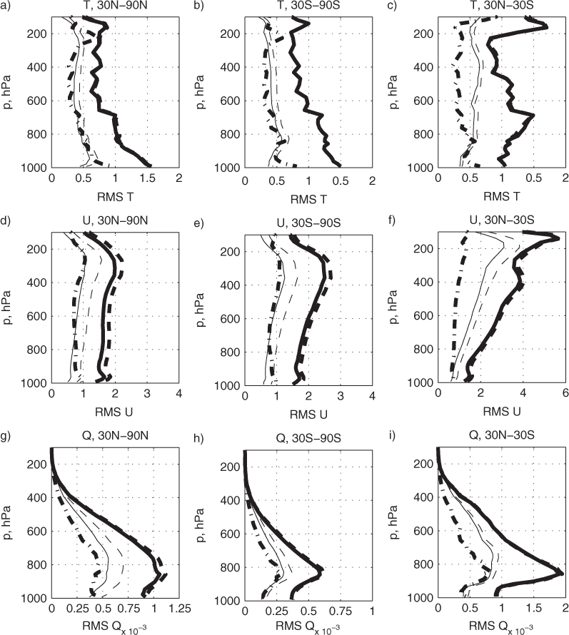
Fig. 1
Global analysis root-mean-square error (RMSE) for July. Left column, 30N–90N; centre column, 30S–90S; right column, 30S–30N. Top row, temperature (K); centre row, zonal wind (m s−1); bottom row, specific humidity (kg kg−1). Solid heavy line, NE experiment; heavy dashed line, Control experiment; heavy dash–dot line, DENSE experiment; thin solid line, Twin NE experiment; thin dashed line, Twin Control experiment.
The smallest analysis RMSE was found in the DENSE experiment, except in the stratosphere and lowest levels of the troposphere where the TWIN NE experiment had the least analysis error. The DENSE experiment has less variation in analysis error with height compared with the Control experiment, the most striking example being the wind error in the tropics. The rawinsonde network in the DENSE experiment has consistent frequency and distribution of sampling throughout the troposphere and lower stratosphere, while the realistic observing network used in the other experiments has very different distributions of observation sampling at different height levels. The analysis RMSE in the DENSE experiment is 50–60% smaller than in the Control in the extratropics, with 60–80% reduction in error in the tropics. The DENSE experiment estimates the limit of improvement of the background state possible using the DAS and forecast model in question if the observing network were nearly ideal, with the caveat that the error covariances are not correctly weighted.
The Twin NE experiment has error close to that of the DENSE experiment for temperature and wind in the extratropics but significantly greater error than the DENSE experiment in the tropics and globally for humidity. The larger errors seen in the tropics and for humidity are believed to be due to convection, which behaves discontinuously and has a short timescale of error growth. A greater increase in analysis error is seen when observation errors are included in the Twin experiments in comparison to the difference between the NE and Control experiments. The analysis error increases by 20–25% in the extratropics and 10% in the tropics for temperature, and by 40% in the extratropics and 20% in the tropics for winds from the Twin NE to the Twin Control experiment.
The time mean analysis error field gives an indication of regions that experience a persistent source of error, which could stem from observation bias or systematic error of the forward model or the DAS. In the OSSE, observation bias should be minimal as no explicit bias was added to the synthetic observations, so any time mean analysis error is likely to stem from model error or data assimilation processes. Time mean analysis error due to systematic model error would result from retention of model error in poorly observed areas, bias correction that incorrectly assumes observation bias in the presence of model error, or weighting of background error that does not account for the systematic error. Systematic errors in the data assimilation process may also result from improper balance assumptions.
Figure 2 shows the monthly mean analysis error for temperature and zonal wind at 500 and 250 hPa, respectively. The DENSE experiment has very little time mean analysis error, indicating that the extensive observational network successfully removes any systematic sources of error. The NE and Control experiments both show significant regions of cold biased analysis temperature, especially in the deep tropics. In these two experiments, systematic model error of the GEOS-5 in comparison to the ECMWF NR is suspected to account for much of this temperature bias. The zonal wind time mean analysis error features strong easterly biases in the eastern Pacific and Atlantic equatorial basins, and westerly bias in the northern Indian Ocean. The easterly biases are due to a known issue with the cross-correlation of background errors of wind and temperature (and therefore to radiance data) by this version of the GSI/GEOS-5. The westerly bias over the Indian Ocean may be due to model error in representation of the upper tropospheric Asian monsoon circulation.
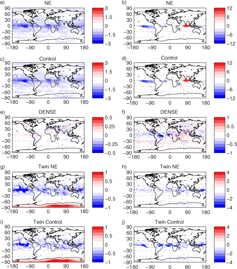
Fig. 2
Monthly mean analysis error on select model surfaces for the experiments in July, longitude on x-axis and latitude on y-axis. Left column, temperature at 500 hPa, K. Right column, zonal wind at 250 hPa, m s−1. Note varying contour intervals between panels.
The Twin experiments also show a cold bias in the deep tropics, but of a much smaller magnitude than in the ECMWF NR experiments. Another region of bias in the Twin bases is located over Antarctica, where a warm temperature bias exists in the analysis field. These biases will be discussed in greater detail in Section 4.
4. Analysis increments
The analysis increment, or analysis minus background, is a measure of the work performed by the DAS in modifying the background field to produce an analysis field x a. The analysis increment can be expressed as:
where the background state x b is adjusted by the ingestion of observations y o using the operation operator H and the gain matrix K. The time mean of the analysis increment indicates the amount of persistent modification of the background. The left column of Fig. 3 shows the zonal mean time mean analysis increment for temperature for the five experiments, and Fig. 4 illustrates the same fields for zonal wind.
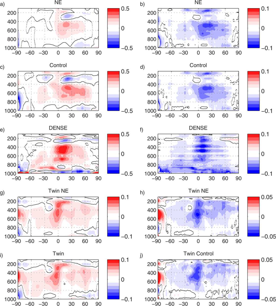
Fig. 3
Zonal mean time mean analysis increment (left column) and MAER (right column) for temperature (K), July, η-level pressure on y-axis and latitude on x-axis. Negative values of MAER indicate an improvement of the analysis field compared to the background. Note different contour range for Twin and ECMWF NR experiments.
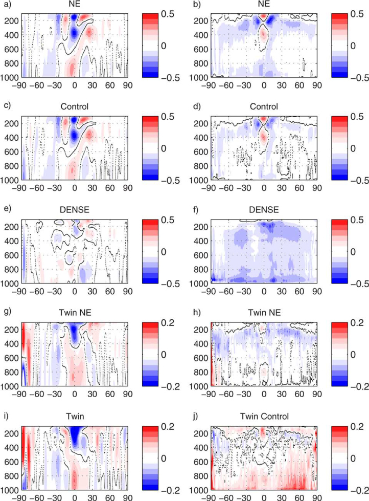
Fig. 4
Zonal mean time mean analysis increment (left column) and MAER (right column) for zonal wind (m s−1), July, η-level pressure on y-axis and latitude on x-axis. Negative values of MAER indicate an improvement of the analysis field compared to the background. Note different contour range for Twin and ECMWF NR experiments.
The analysis increment gives a measure of work done by the observations, but does not indicate whether this work is beneficial, harmful or neutral to the analysis quality. The difference between the absolute value of analysis error and absolute value of background error, denoted here as ‘mean absolute error reduction’ (MAER), gives an indication of whether the analysis increment is performing useful work or not, with negative values indicating an improvement of the analysis compared to the background. The zonal mean time mean distribution of MAER for temperature is shown on the right columns of Figs. 3 and 4. For most regions, MAER is negative, with the analysis having less error than the background.
The largest time mean positive analysis increments for temperature are found in the tropics in areas of deep convection. Large negative time mean MAER is seen in the tropics for temperature, indicating that the time mean analysis increments are acting to remove errors from the background. These time mean analysis increments correspond to the regions of time mean analysis error seen in Fig. 2. The Twin experiments have smaller increments than the ECMWF NR experiments (note the different contour intervals).
Examination of the analysis increments helps diagnose some of the analysis temperature biases found in the two Twin experiments. In the Antarctic region, the ingestion of observations has a detrimental effect on the temperature field, indicated by the positive values in the middle troposphere in this region (Fig. 3h and j). There are known difficulties with the use and generation of radiance observations in this area due to the elevated, snow-covered surface and presence of cloudy regions during polar night, even in this OSSE context.
A different mechanism causes the cold analysis temperature bias in the Twin experiments. For these experiments, a positive temperature analysis increment acts to improve the analysis state in comparison to the background state, indicating that biases of the observations are not responsible for the analysis temperature bias. If a temperature bias persists for a long period in this scenario, the ‘forcing’ due to the analysis increment to increase temperatures must be equal to a different ‘forcing’ of opposite sign driven by model processes or interactions between the model integration and the DAS. Diagnosis of the model behaviour in these experiments is particularly difficult due to the use of incremental analysis updates (IAU) by the GSI, and the IAU is itself a likely source of this persistent cold bias in the analysis.
Figure 5 shows the zonal mean temporal variances of the analysis increment for the five experiments. While the time mean analysis increment primarily illustrates the removal of systematic background error by the observations, the variance of the analysis increment illustrates the role of non-systematic errors. Variance of the analysis increment is influenced both by the observation error directly [as in eq. (1)] and through the growth of ingested observation errors from previous cycles. The Control experiment has larger analysis increment variance than the NE experiment as a result of these two factors.
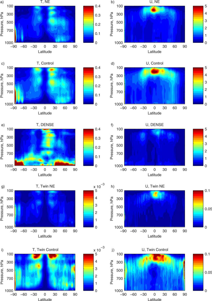
Fig. 5
Zonal mean variance in time of the analysis increment for temperature (K2), left, and zonal wind (m2 s−2), July mean.
While the Control experiment has larger time mean and variance of analysis increments than the NE experiment, the MAER field shows that the useful work done by the observations in both experiments is nearly the same. In a stable DAS, the work done by ingestion of observations should be equal to the growth of errors between cycle times. This error growth is a function of the chaotic nature of the model dynamics and physics, the model error, and the initial analysis error; the first two are identical in the two experiments. As seen in Fig. 1, there is also little difference in the analysis error between the NE and Control experiments for temperature, so it is not surprising that the error growth rate in the two experiments should be nearly the same.
The NE and Control experiments feature regions of wind field quality degradation by the assimilation process on the equator in the middle and upper troposphere, due to improper balancing of radiance observations (a known issue with this version of GEOS-5/GSI). This degradation is not observed in the DENSE experiment, where only rawinsonde observations with paired temperature and wind observations are ingested. The Twin NE experiment also shows some degradation of the analysed wind field at the equator, although this is predominantly in the lower troposphere.
There is little difference between the Twin NE and Twin Control for either time mean analysis increment or MAER for temperature but a significant difference in MAER for zonal wind. While the Twin NE experiment shows improvement of the background state due to the DAS, the Twin Control experiment shows degradation of the background state in the mid and lower troposphere due to the presence of observation errors. The Twin Control experiment has larger variances of analysis increment than the Twin NE experiment, although the variances of both Twin experiments are an order of magnitude smaller than for the ECMWF NR experiments. The increase in error variance relative to the Twin NE experiment is much greater than the relative change for the ECMWF NR experiments. In the Twin experiments, the observation errors and their growth are large compared to other sources of error, while in the ECMWF NR experiments model error is a significant additional source of error.
The DENSE experiment has the largest time mean analysis increments and MAER of all experiments, due to the quantity and distribution of observations. The low analysis errors in the DENSE experiment are maintained by persistent ingestion of observations that work to counteract the growth of model and initial condition errors. The observations have no added errors and are so dense that the simplified statistically defined background and observation error covariances that determine the spread of information in the DAS do not degrade the accurate information provided by the observations. Also, the use of reduced observation error covariances by the GSI in the DENSE experiment causes the analysis to draw more strongly to the observations.
The MAER field for temperature in the DENSE experiment shows horizontal striations that are not present in the analysis increment field. These striations are due to differences in the vertical interpolation of the rawinsonde observations in comparison to the NR verification field interpolation, illustrating an aspect of implicit representativeness error in the synthetic observations. The larger MAER in the lower troposphere in the DENSE experiment compared to the NE and Control experiments results because the observations remove systematic model error from the analysis in the DENSE experiment that is retained in the NE and Control experiments.
The greatest variances of analysis increment in the DENSE experiment occur in different regions compared to the other experiments. For the DENSE experiment, the variance of the analysis increment indicates the region with the fastest growing errors – in this case, near the intertropical convergence zone (ITCZ) and near the surface. In the Control and NE experiments, there are not always sufficient observations in these regions to incur a large analysis increment. Instead, errors in these poorly observed regions may be retained by the DAS in the Control and NE experiments, with greater analysis increments in other regions that have additional observations.
There is less difference between magnitudes of the background RMSEs for the Control and NE experiments than between values for the two analysis RMSEs. This implies that during the forecast period that creates the backgrounds from the analyses, a large portion of the additional analysis error created by observation error actually decays. Multiple processes may be responsible for this decay, including explicit and implicit diffusion or damping, that on small spatial scales may be quite rapid. Also, wave dispersion can reduce error maxima and even cause error variances to be exchanged between fields, as happens during geostrophic adjustment. The latter process also can be significant on a timescale of a few hours. Other less well-understood processes may be at work, such as those responsible for the dominance of error decay reported by Errico et al. (2001) for a different model.
5. Forecast errors
Forecast error can be calculated explicitly using the NR as verification. The RMS forecast errors at 24 and 120 hours are shown for the month of July in Figs. 6 and 7, for temperature and zonal wind, respectively. Although the DENSE experiment has lowest error at the analysis time, by 24 hours the error in the DENSE experiment has increased significantly and generally matches or exceeds the error in both Twin experiments. At 120 hours, the RMSE for the DENSE experiment is much smaller than in the Control and NE experiments, but the Twin experiments have the smallest forecast RMSE. The wind and temperature fields show greater forecast RMSE in the Southern hemisphere extratropics compared to the Northern hemisphere extratropics, including for the DENSE experiment in which there is no hemispheric difference in the observing network. The greater errors in the Southern hemisphere may be due to the seasonal differences or topographic differences between the Northern and Southern hemispheres.
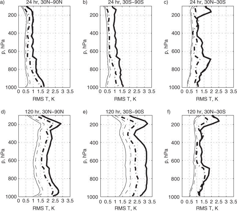
Fig. 6
Forecast root-mean-square error (RMSE) for temperature, July mean. Left column, 30N–90N; centre column, 30S–90S; right column, 30S–30N. Top row, 24 hour forecast; bottom row, 120 hour forecast. Solid heavy line, NE experiment; heavy dashed line, control experiment; heavy dash–dot line, DENSE experiment; thin solid line, Twin NE experiment; thin dashed line, Twin Control experiment.
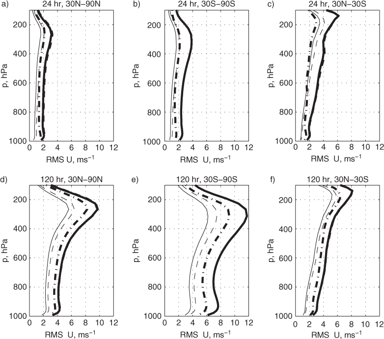
Fig. 7
As for Fig. 6, but for zonal wind u, m s−1.
In the tropics, physical processes play a large role in forecast error. The wind and temperature RMSEs show relatively little spread between the five experiments at 120 hours although there is large spread at the analysis time. The lack of spread of error at 120 hours suggests that the forecast errors of wind in the tropics are not dominated by differences in model climatologies but by more intermittent processes such as convection. The temperature RMSEs in the tropics show more spread between the Twin experiments and ECMWF NR experiments in the lower troposphere, indicating that model error plays a larger role at those levels.
The Twin experiments demonstrate a marked impact of observation error on the RMSE forecast error that persists from the analysis time to the 120-hour forecast. This is in contrast to the Control and NE experiment pair, where the initial difference in the two experiments at the analysis time diminishes so that there is nearly-identical RMSE at 120 hours in the tropics and Northern hemisphere extratropics (the lines in Fig. 6 are nearly-completely overlain), and only minimal difference in the Southern hemisphere extratropics.
5.1. Error growth rates
The forecast error variances (calculated as true variance with temporal biases removed) are shown in Fig. 8 for 250 hPa wind and 500 hPa temperature as a function of time, with semi-log scaling of the variance to allow easy comparison of growth rates. If exponential growth of error variance is assumed [see eq. (A1) in the Appendix], the slope of the temporal curve of the logarithm of variance will give the growth rate. All five experiments have error variance curves that are roughly parallel after the first 48 hours of forecast; however, the error variance growth during the first 24 hours differs significantly between experiments.
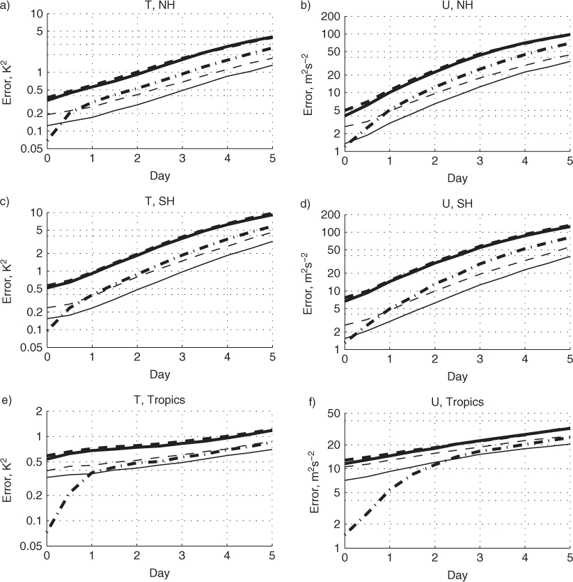
Fig. 8
Global error variance as a function of forecast time, July mean. Left column, 500 hPa temperature (K2); right column, 250 hPa zonal wind (m2 s−2). Top row, 30N–90N; centre row, 30S–90S; bottom row, 30N–30S. Solid heavy line, NE experiment; heavy dashed line, control experiment; heavy dash–dot line, DENSE experiment; thin solid line, Twin NE experiment; thin dashed line, twin control experiment.
The fastest initial growth of error variance is observed for the DENSE experiment, particularly in the tropics. The second fastest initial error growth is seen in the NE experiment, but the DENSE experiment growth rates are considerably higher than the NE growth rates. Maps of differences between the 12-hour forecast and analysis error variances (Fig. 9) illustrate the spatial distribution of error growth. In the DENSE experiment, error variances grow rapidly over areas of deep convection in the tropics and summer hemisphere as well as the winter hemisphere storm track. A test was performed using the observational network from the DENSE experiment in the Twin OSSE framework for comparison, and rapid error growth was not observed during the first 2 d of the forward integration. These test results in the Twin setup imply that the primary cause of the rapid initial error growth in the DENSE experiment is model error.
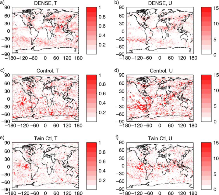
Fig. 9
12-Hour forecast error variance minus the analysis error variance for the month of July. Left column, temperature variance (contour interval 0.1 K2) on model surface nearest 500 hPa; right column, zonal wind variance (contour interval 1.5 m2 s−2) on model surface nearest 250 hPa. x-axis, longitude; y-axis, latitude. Top, DENSE experiment; centre, Control experiment; bottom, Twin Control experiment.
In the Control and NE experiments, large regions degraded by model error remain in the analysis state. Compared with the DENSE experiment, the pattern of error variance growth during the initial forecast period seen in Fig. 9 is more spatially uniform and not focused in convective regions. Instead, regions of fast error variance growth include the eastern Pacific basin and the South American and African continents.
By day 2 of the forecast, the initial condition errors that project onto damped modes have been greatly reduced and similar dynamics governs the dominant error growth. The rapid initial error growth in the DENSE experiment slows dramatically after 24–36 hours of forward integration. The similarity in growth rates during this period implies that additional model error is not contributing significantly to error variances during this time.
After day 4, the growth rates for the Control and NE experiments begin to slow in the extratropics, while there is little change in the DENSE or Twin experiments. After a period of exponential error growth, the error begins to saturate at longer forecast times (Lorenz, 1982). The slight decrease in error variance growth rate in the Control and NE experiments may be the beginning of the error saturation regime. Because the Twin and DENSE experiments have error variances that lag behind the Control and NE experiments, the Twin and DENSE experiments are further from error saturation at day 5 and do not show a reduction in error growth rate.
The change in forecast skill is equivalent to an improvement in forecast lead time of approximately 12 hours for the Twin NE experiment compared to the Twin Control experiment. This improvement is maintained through the 120-hour forecast period. Similarly, the DENSE experiment shows an improvement of approximately 24 hours in the extratropics, and 2–3 d in the tropics compared to the Control experiment, which is also maintained through the entire forecast period. There is very little improvement in the NE experiment compared to the Control experiment after the first 24 hours of forecast period.
Doubling times for the RMS forecast errors of temperature and zonal wind are calculated using the 48 to 96-hour forecast period to estimate the error growth rate. These doubling times are listed in Table 2. The doubling times were calculated using the simple relation in eq. (A3) in the Appendix. This relation neglects model error and error saturation terms, assuming a simple exponential growth of RMSE. For the forecast period from 48 to 96 hours, this assumption of exponential growth gives a relatively good fit to the actual error growth.
Table 2. Doubling times in days for RMSE of temperature and zonal wind, calculated using a fit to forecast error from 48 to 96 hours
NHSHTropicsNHSHTropics
Control2.82.310.72.62.67.7NE2.52.310.72.42.66.9DENSE2.52.07.72.22.04.8Twin Ctl2.82.39.22.52.37.7Twin NE2.52.08.22.22.16.9
The doubling times are very similar for the two Twin experiments and the DENSE experiment, with slightly longer doubling times for the Control and NE experiments for wind. Doubling times are considerably longer in the tropics than in the extratropics. The doubling times calculated here are longer than the doubling times of 500 hPa geopotential height found by Simmons and Hollingsworth (2002), but this is due to the use of temperature and wind on η levels rather than geopotential height: the latter is a vertically integrated metric that effectively measures more of the barotropic component of the error. The barotropic error modes are known to grow more rapidly than baroclinic error components (Errico, 2000).
5.2. Observation error impacts
If two sources of error are independent, then the total error variance of the combined errors is simply the sum of the variances of both types of error. Because the observation errors that are deliberately applied to the synthetic observations are not correlated with the background or model errors, the error variance of the analysis state due to the ingestion of observation errors may be calculated by subtracting the total analysis error variance of the experiment with no applied observation error from the analysis error variance of the corresponding experiment that includes added observation errors. This result is also valid for the impact of observation errors on the forecast error variance if errors introduced into the forecast by independent observation errors also remain uncorrelated during the forward integration process; this will generally only hold as long as the error dynamics are linear.
Figure 10 shows the ratio of the areal mean error variance of the Control to the areal mean error variance of the NE experiments for both pairs of experiments for the two NRs. In the absence of model error, if the growth rate of the error variance stemming from observation errors is the same as the growth rate of the error variance arising from other sources of error, this ratio should remain constant during the forecast integration. The Twin experiments, having no model error, only show a nearly-constant ratio of error variances for the temperature field in the Southern Hemisphere and for both zonal wind and temperature in the tropics. For other variables and regions, the ratios of error variances for the Twin experiments approach one as the forecast time increases.
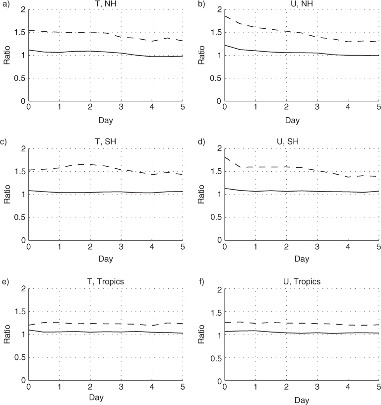
Fig. 10
Ratio of areal mean error variances as a function of forecast time between the Control and NE experiments (solid line) and between the Twin Control and Twin NE experiments (dashed line), July. Top row, 30N–90N; centre row, 30S–90S; bottom row, 30N–30S. Left column, ratio for temperature at 500 hPa; right column, ratio for zonal wind at 250 hPa.
It is expected that only a fraction of the errors present at the analysis time will project onto growing modes, while the rest will project onto damped modes. If the fraction of observation errors that project onto growing modes is small, then the ratio of error variances will approach one during the initial forward integration. Reduction of initial condition errors is expected to occur rapidly over the first day or two of the forecast, reflected in the initial decrease in the ratio of variances noted for zonal wind in the extratropics. However, the ratio continues to decline through the entire 5-d forecast period. This indicates that the timescale for the damping of initial errors is at least several days, and/or that the error growth behaves nonlinearly.
When model error is present, as in the Control and NE experiments, it is not expected that the ratio of error variances in the two experiments will remain constant during forward integration due to the growth of model error. Error variances due to model error will have a very different growth rate with multiple timescales compared to the growth rate of errors stemming from initial condition error. Because model error is defined to be zero at the analysis time (although the background error and thus analysis errors are likely to be correlated with systematic model error), an increase in model error variance with time will result in the ratio of variances of the Control and NE experiments tending towards unity.
6. Discussion
When a numerical weather prediction model with data assimilation is cycling in a stable regime, where the errors of the analysis field are not persistently increasing or decreasing, there must be a balance between the growth of errors between cycle times and the ‘work’ done by ingestion of observations to improve the analysis compared to the corresponding background state (Daley and Menard, 1993). The error growth between cycles depends on the behaviour of model error and initial condition errors, with the initial condition errors themselves influenced by observation error, inaccuracies in the DAS process and background errors accumulated during previous model cycles. Some of the initial condition errors project onto growing modes, while a large fraction projects onto damped modes. Model error has a complex growth rate as it consists of error processes with different timescales, including fast physical processes such as convection and numerical filtering, as well as slower dynamical and physical processes.
In the identical twin experiments, the fields of analysis error and analysis increment illustrate the regions of the globe that are constrained by assimilation of observations, as well as those that are not. The tropics are found to have the greatest variance and mean analysis error in the identical twin experiments, with the least error over the continental United States and western Eurasia.
Due to imperfections in the data assimilation process and representativeness errors inherently present in the synthetic observations, errors will be introduced into the Twin NE fields even when initialising from a ‘perfect’ background field. Even in experiments where an ingested observation locally improves the analysis state compared to the background, the resulting analysis state may be dynamically or physically unstable such that the forecast model will then amplify the error. This type of behaviour is seen for temperatures in the tropics in both Twin cases, where the analysis increments act to improve the analysis compared to the background, but interplay between the DAS and the model nevertheless results in a cold bias.
The impact of initial condition errors on forecast accuracy is explored in these experiments. The DENSE experiment can be considered a ‘best observing network’ scenario, where the initial condition error is minimised within the current data assimilation framework. A true ‘perfect initial condition’ state does not actually exist because the ECMWF NR cannot be completely or perfectly represented using the GEOS-5 model due to differences in model grids and representation of parametrisations and variables. Initial attempts to approximate the ECMWF NR state directly on the GEOS-5 grid met with technical difficulties such that the resulting initial state would likely be no more accurate than the analysis states of the DENSE experiment. Instead, the DENSE experiment was chosen as a suitable alternative to study the role of initial condition errors.
Rapid growth of model error is clearly illustrated in the DENSE experiment during the first 24 hours of forward integration. This rapid error growth is not seen in the Twin experiments that have initial condition error of similar magnitude in the extratropics, implying that this error growth is most likely due to model error. The analysis errors in the DENSE experiment are very low due to the strong constraint of the global rawinsonde network, and thus the initial state is very close to the ECMWF NR state but in considerable disagreement with the preferred climatology of the GEOS-5 model. In the Control and NE experiments, the relative sparseness of the observational network allows the analysis state to retain more of the GEOS-5 systematic model error with respect to the ECMWF NR, so that much less adjustment towards the GEOS-5 preferred climatology occurs during the early forecast period.
While it is desirable to attempt to quantify exactly the growth of model error and initial condition errors in conjunction with a simple theoretical framework of error growth, there are limitations to the practical application of such simplified theory to the experimental results. An attempt was made to fit the error growth rates to the simple model of exponential initial condition error growth with constant model error growth, as in Leith (1978). However, the fit of the data to theory was poor and did not yield useful estimates of model error growth rates.
Instead, some general statements quantifying model error growth in relation to initial condition error growth can be made. The results show that for the GMAO OSSE system, model error is dominant over initial condition error for medium-range forecasts. The very rapid error growth observed during the first 24–48 hours of forward integration in the DENSE experiment is caused by model error, rather than growth of small initial condition errors. This sets a strict limit on the possible improvement in forecast skill to be achieved by reduction of initial condition errors, with the best possible improvement in forecast lead times being on the order of 24–36 hours for medium-range forecasts. The Twin experiments have improved forecast skill of approximately 2 d in the extratropics and more than 3 d in the tropics compared with the Control, indicating that more significant gains in forecast skill are possible with improvements to the forward integrating model. It should be noted that the nature of model error growth in this case is actually a comparison of the ECMWF forecast model (circa 2005) with the GEOS-5 forecast model, and not a true comparison of the GEOS-5 model with the real world.
7. Acknowledgments
The OSSE was conducted with the assistance of Ricardo Todling, Meta Sienkiewicz, King-Sheng Tai and Joseph Stassi at the GMAO. Erik Andersson provided the ECMWF NR through arrangements made by Michiko Masutani. Support for this project was encouraged by Michele Rienecker and provided by GMAO core funding. The authors also thank three anonymous reviewers for their helpful comments.
Appendices
8. Appendix
A basic sense of how initial condition and model error act together to produce forecast error is revealed by considering a simple one-component model of linear dynamic growth with an added external forcing. Consider an error x governed by:
where t is time, λ is a growth rate due to linearised error dynamics and f(t) is the external forcing. The latter represents model error due to imperfect formulation, independent of the forecast error itself. The general solution to (A1) is
First, consider the case when f(t) is time independent with . Then
The first term describes the result of initial condition error and the second of model error. Both have an exponential component, indicating that as model error creates forecast error, the same dynamics apply, yielding the same growth rate. For short forecast times (t<<1/λ), however, the forecast error growth due to model error is dominated instead by the addition of model error rather than dynamic growth of previously added model error. The effect of model error is only seen after the error has had sufficient time to act, unlike the effects of initial condition error that may be seen immediately. At longer forecast times the dynamic growth of earlier added model error dominates the effect of such error still being added and, at such times, it is difficult to distinguish the presence of initial condition and model error based on the temporal behaviour of the error alone.
If a set of independent cases are considered for which the means of the initial condition and model errors are zero and the variances are V(0) and F, respectively, with no correlation between the two types of error, then the variance of the forecast error as a function of time, computed by averaging over all the cases, is
If the forcing is instead stochastic white noise, with F s indicating its variance, then
The very similar forms of eqs. (A4) and (A5) reveal that similar comments about dynamics acting on previously applied model error in the case of time-independent forcing apply. Since white noise and temporally constant forcings can be considered somewhat as extremes, their similar results provide confidence of the generality of the results for other likely types of forcing.