
Table 1. List of observables and description of the sensors characteristics
Sète stationAir pressureVaisala-PTB2203600 s0.5 hPaPrecipitationPrécis Mécanique – PM 3030 tipping bucket rain gage 1000 cm2360 s0.2 mmMarseillan tableWind speed and direction (6 m)Young – Wind monitor 051032 s–60 s average0.3 m s−1 – 3 °Air temperature (4 m)Atexis – platinum wire 1000 Ohm/class A. Socrima radiation shield10 s–60 s average0.5°CAir humidity (4 m)Vaisala – HMP45 hygrometer. Socrima radiation shield10 s–60 s average3%Longwave and shortwave radiationKipp and Zonen – CNR1 radiometer10 s–60 s average10% of daily totalWater temperature (−10 cm)Atexis – Platinum wire 1000 Ohm/class A10 s–60 s average0.1°CWater temperature profileChauvin Arnoux – Platinum wire 100 Ohm class A10 s–60 s average0.1°CFast-response temperature (5 m)Gill – HS50 sonic anemometer25 Hz0.05°CFast-response 3D wind (5 m)Gill – HS50 sonic anemometer25 Hz0.01 m s−1Fast-response water vapour (5 m)Licor – 7500 infrared gas analyzer20 Hz0.1 g kg−1TurbidityYSI-66001800 s2%Ifremer boatRadio-sounding (0–4000 m)Vaisala – RS92SGP
– Humidity
– Temperature
– Pressure
– Wind speed
– Wind direction
2 s/10 m
5%
0.5°C
1 hPa
0.15 m s−1
2°CSurface reflectance and solar irradianceSpectroradiometer – FieldSpec UV/VNIR (ASD)1800 s–3600 s3 nm /
5% from 400–900 nmInwater solar radiance profileSpectroradiometer – FieldSpec UV/VNIR (ASD) + optical cableApprox. 9000 s3 nm /
5% from 400–900 nmTurbidityHACH – 2100 N ISOn request2%
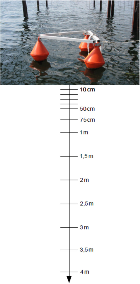
Fig. 1
Device for measuring the temperature profile. The picture shows the device structure and the measurement depths from 10 cm to 4 m are indicated below.
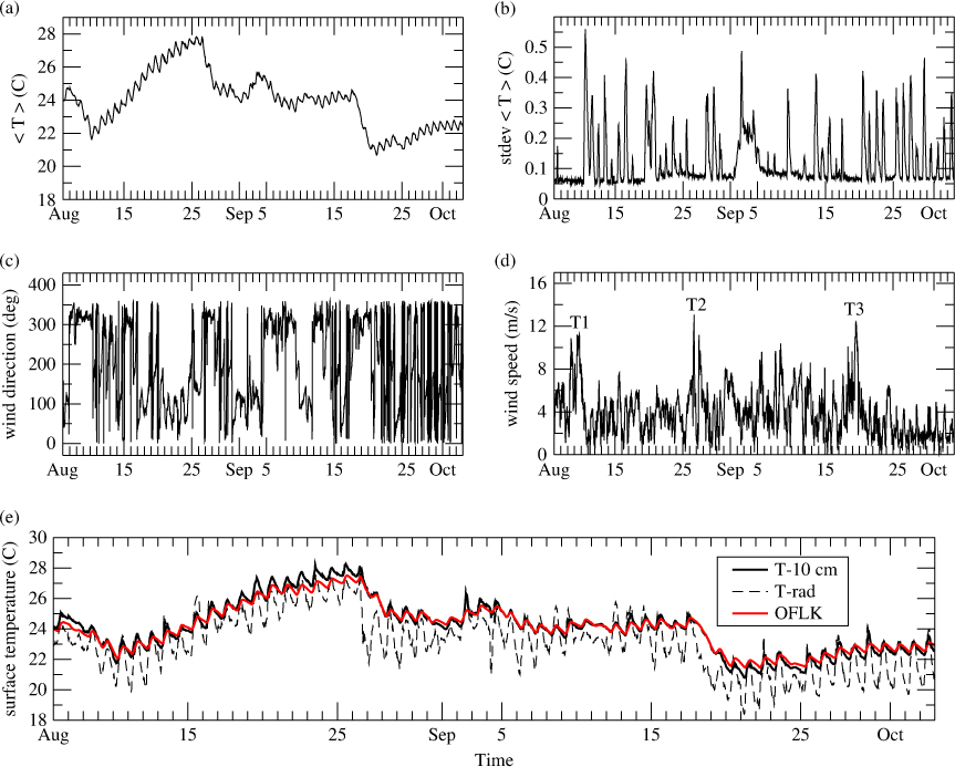
Fig. 2
For the THAUMEX period: (a) vertical mean water column temperature <T>, (b) standard deviation of <T>, computed from profile measurements. Measured wind direction (c) and wind speed (d), T1, T2 and T3 indicating the Tramontana events. (e) 3 Hourly running average of temperature measured at −10 cm (solid black), radiative temperature calculated from radiation measurements (dashed black) and surface temperature modelled with the OFLK calibrated FLake configuration (red).
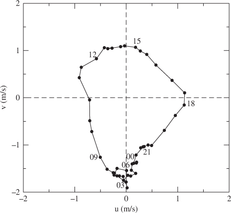
Fig. 3
Hodograph of daily mean wind over the THAUMEX period. Numbers indicate UTC times.
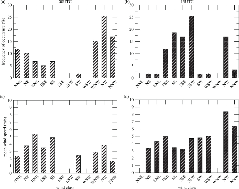
Fig. 4
Histograms of frequency of occurrence at 00 UTC (a) and 15 UTC (b) and mean wind speed at 00 UTC (c) and 15 UTC (d) for wind classes where direction was divided into 12 sectors of 30° each.
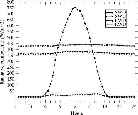
Fig. 5
Average daily cycle of radiative components: shortwave downward (SWD) and upward (SWU), longwave downward (LWD) and upward (LWU), measured at the Marseillan table.
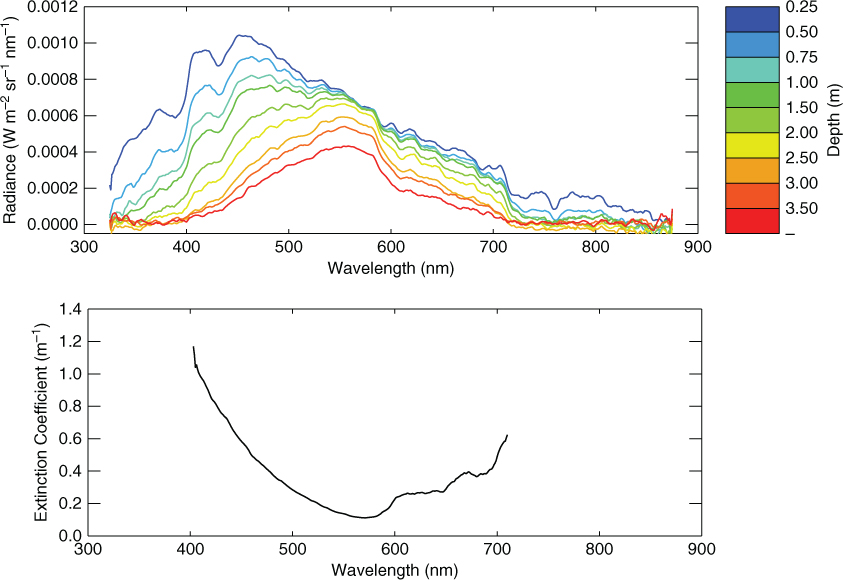
Fig. 6
(a) Measurements of underwater spectral radiance at several levels deep taken from the IFREMER boat at the Marseillan table for IOP1 (1745 local time) and (b) spectral extinction coefficient obtained from these measurements.
Table 2. PAR extinction coefficients calculated through eq. (3) for IOP1 (24 August 2011)
2011/08/24 – 08:30Marseillan0.882011/08/24 – 12:30Bouzigues0.532011/08/24 – 15:30Bouzigues0.312011/08/24 – 17:45Marseillan0.37
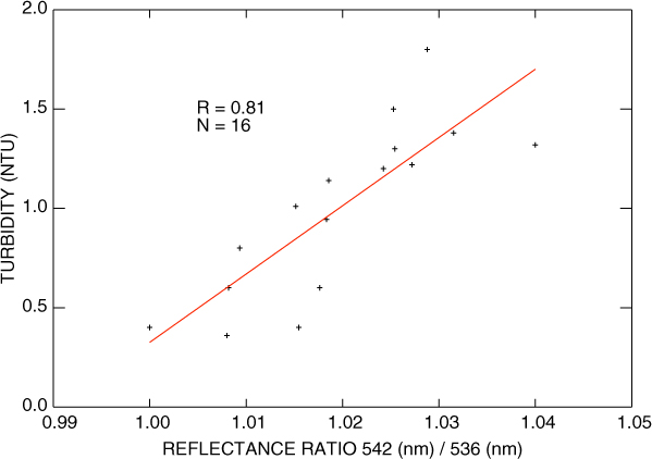
Fig. 7
Scatter plot between field water-leaving reflectance ratio (542/536 nm) and water turbidity (turbidimeter type: HACH 2100N) for IOP2.
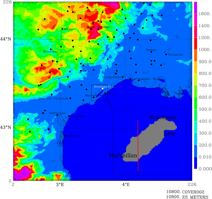
Fig. 8
Simulation domains located in the south of France at the Mediterranean Sea. The bigger domain shows the orography of the area, with the Mediterranean coastline (black line) and the lake contours (thin black line), whereas the limits of the 200-m resolution domain are represented in a square, zoomed on the bottom-right part of the figure, in which the north–south oriented red line represents the axis of the vertical cross-section. Black dots correspond to the stations of the French observation network (only a few names are indicated).
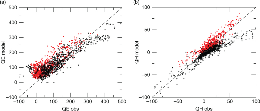
Fig. 9
IOP2 scatter plot (a) of latent heat flux (QE) for observations (OBS) and model (OFLK) during the day (black dots) and night (red dots); scatter plot (b) of sensible heat flux (QH) for observations (OBS) and model (OFLK) during the day (black dots) and night (red dots).
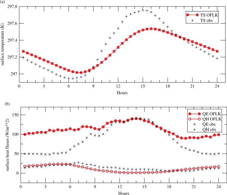
Fig. 10
Average daily cycle for observations (OBS) and model (OFLK), of surface temperature (a) and surface latent and sensible heat fluxes (b).
Table 3. Energy budget components (W m−2) averaged over the whole period for the observations (OBS), the model (OFLK) and the experiment where surface temperature derived from radiation measurements is used instead of model surface temperature (DIAG)
DayOBS1712984577−6OFLK16729706330DIAG1712984582−2NightOBS−290−8423725OFLK−310−804270DIAG−290−8433319TotalOBS14129−4821321OFLK13529−12108100DIAG14129−493518
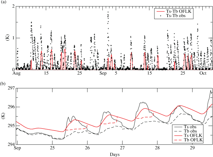
Fig. 11
(a) Time evolution of the difference between surface (T s ) and bottom temperature (T b ) in the model (OFLK) and the observations (OBS), (b) modelled (solid red) and observed (T s ) (solid black), modelled (dashed red) and observed (T b ) (dashed black) over a 4-d stratified period.
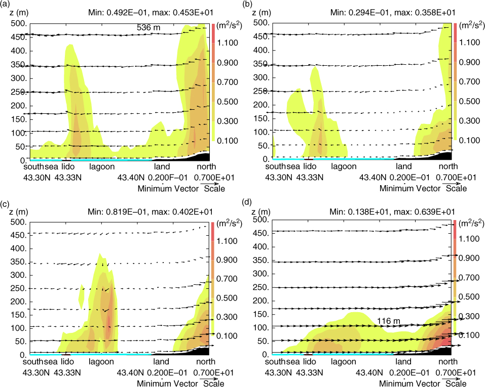
Fig. 12
Vertical cross-section of TKE superimposed onto wind during IOP2. (a), (b), (c) and (d) correspond respectively to 09, 10, 11 and 12 UTC. Numbers on (a) and (d) correspond to the observed ABL height.
Table 4. Boundary layer height (m) measured and modelled at 09 UTC, 12 UTC and 15 UTC
Observations536116103MFLK39979107MNLD295107107
Table 5. IOP2 3-hourly averaged biases and RMSEs computed from 90 meteorological stations over land between 06 UTC and 18 UTC for 2 m temperature, relative humidity and the components of 10 m wind, using MFLK model configuration
Mean bias−0.141.12−0.38−0.32Mean RMSE2.2611.762.262.74
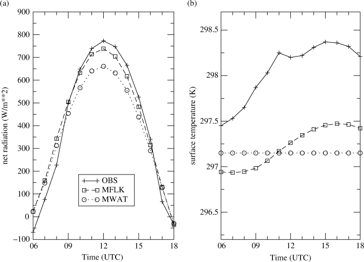
Fig. 13
Net radiation (a) and surface temperature (b) observed (solid line with crosses), modelled by MFLK (dashed line with squares) and by MWAT (dotted line with circles), for IOP2.
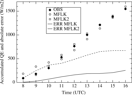
Fig. 14
Time evolution of accumulated latent heat flux QE (symbols) and associated absolute error for the model (ERR MFLK) and the 2-hour shifted model (ERR MFLK2).
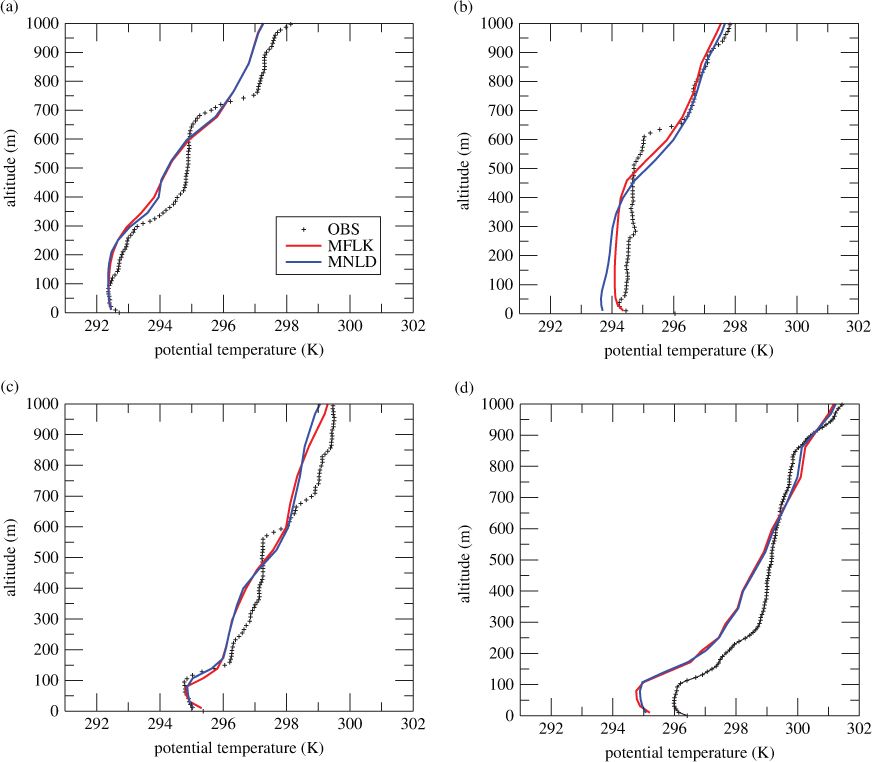
Fig. 15
Potential temperature profiles at 07, 09, 12 and 15 UTC. The crosses is radio-sounding, red line corresponds to MFLK and blue to the MNLD experiment.