Fig. 1.
Projection on the WRF outer domain of vertical velocity (colour) and horizontal winds (arrows) in m s−1, computed with ECMWF operational analyses at 5000 m altitude on 1800 UTC 6 October 2005. The vertical velocity scale is given by the coloured bar to the right and the wind scale by the arrow at the bottom right corner. Black contours indicate the coast of the Antarctic continent and South America. The black box around the Antarctic Peninsula gives the location of the inner domain used in the WRF simulation, which is also the domain used in the domain- and box-averaged budget analysis of Figs. 9–14.
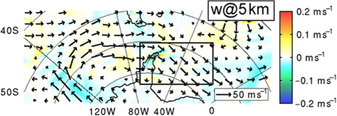
Fig. 2.
As in Fig. 1, except for the pressure in hPa at isoaltitudes 15000 m (a), 25000 m (b) and 35000 m (c).
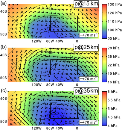
Fig. 3.
Terrain elevation (m) of the inner domain used for the WRF simulation with orography. The height scale is given by the coloured bar to the right. The curved black line delimits the coast of the Antarctic Peninsula and off-shore islands. The straight black line (A–B) gives the location of the vertical cross-sections in Fig. 6.
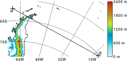
Fig. 4.
Horizontal cross-section at 5-km altitude of vertical velocity (colour) and horizontal winds (arrows) in m s−1, computed from the inner domain outputs of the WRF modelling experiment with orography on 1800 UTC 6 October 2005. The vertical velocity scale is given by the coloured bar on the right side and wind scale by the arrow on the bottom right corner of the panel. The straight black line (A–B) gives the location of the vertical cross sections in Fig. 6.
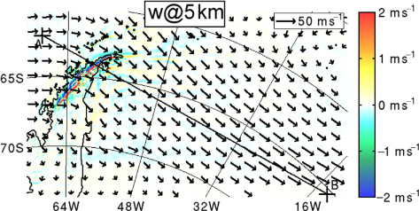
Fig. 5.
(a) As in Fig. 4, except for the vertical velocity in m s−1 at 30 km altitude. (b) As in (a), except for the x-component of the wind in m s−1. (c) As in (a), except for the y-component of the wind in m s−1 at 30 km altitude. (d) As in (a), except for the static stability in s−1. (e) As in (a), except for the Richardson number. (f) As in (a), except for the potential vorticity in pvu.
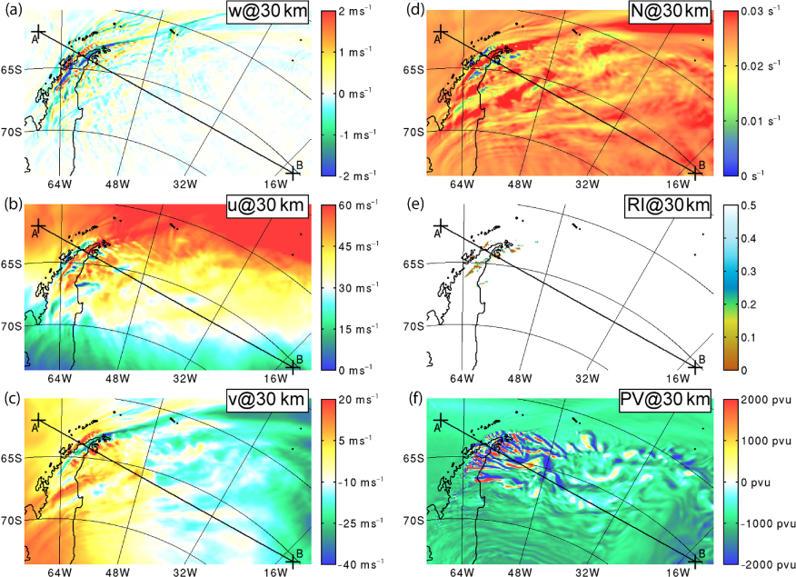
Fig. 6.
(a) Vertical cross section of the vertical velocity (colour) in m s−1 and the isentropes (black contours) in K, computed from the inner domain outputs of the WRF modelling experiment with orography at the location indicated by line (A–B) in Figs. 3–5 on 1800 UTC 6 October 2005. The horizontal axis gives the horizontal coordinate in (latitude, longitude) and the vertical axis on the left-side (right side) gives the altitude in m (the potential temperature in K). The profile of the Antarctic Peninsula ridge is shaded in black. (b) As in (a), except for the x-component of the wind in m s−1. (c) As in (a), except for the y-component of the wind in m s−1. (d) As in (a), except for the static stability in s−1. (e) As in (a), except for the Richardson number. (f) As in (a), except for the density times potential vorticity in pvu kg m−3.
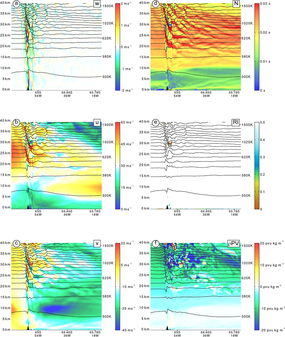
Fig. 7.
(a) Time–height diagram of u in m s−1 from the 20-min inner domain outputs of the WRF model experiment with orography, domain-averaged in the inner domain (see the domain delimited by the black rectangle in Fig. 1). The horizontal axis gives the time in hours from 0000 UTC 6 October 2005 to 0000 UTC 7 October 2005 and the vertical axis gives the height in m. The wind scale is given by the coloured bar on the right hand of the panel. (b) As in (a), except for v in m s−1. (c) As in (a), except for KH in J kg−1. (d) As in (a), except for the so-called differential u calculated as the difference between outputs from the WRF model experiments with and without orography. (e) As in (d), except for differential v. (f) As in (a), except for differential KH.
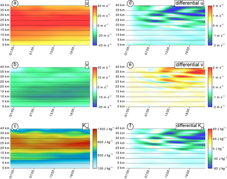
Fig. 8.
(a) Time evolution of differential u (red line) and differential v (green line) calculated as a difference between the 20-mininner domain outputs from the WRF simulations, with and without orography, after domain averaging in the inner domain and vertically averaging between 0 and 40 km. The horizontal axis gives the time in hours from 0000 UTC 6 October 2005. The vertical axis gives the intensity in m s−1. (b) As in (a), except for KH from the WRF experiment, with orography (red line) and without orography (green line) in J kg−1.
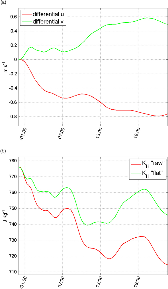
Fig. 9.
(a) As in Fig. 7a, except for Fu. (b) As in (a), except for Fv. (c) As in (a), except for XGW. (d) As in (a), except for YGW.
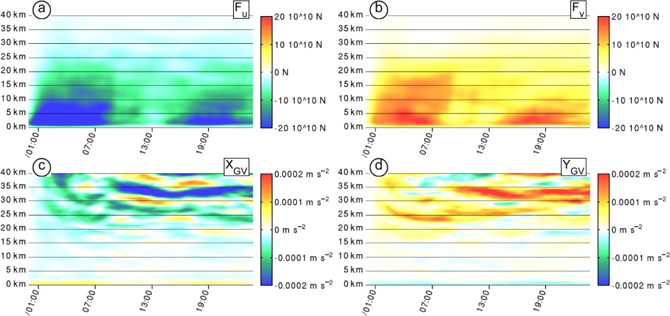
Fig. 10.
As in Fig. 7, except for the difference of the terms of the budget of u in m s−2: (a) tendency, (b) sum of the source terms, (c) sum of the Coriolis and pressure forces, (d) total-flux divergence, (e) Coriolis force, (f) horizontal flux divergence, (g) pressure force, (h) vertical flux divergence, (i) friction and (j) residual term.
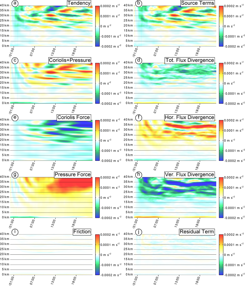
Fig. 11.
As in Fig. 10, except for the budget of differential v.
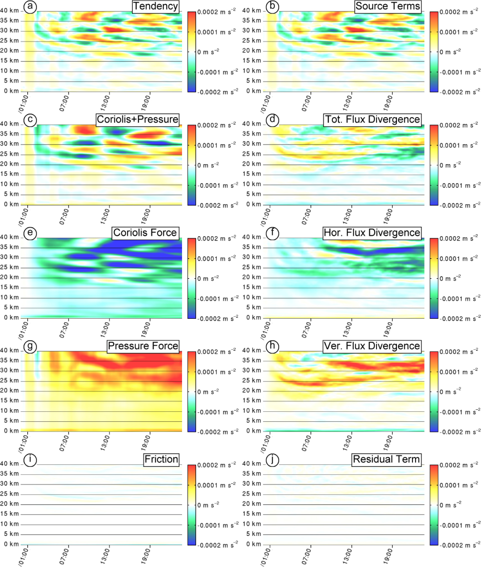
Fig. 12.
(a) As in Fig. 8a, except for the terms of the budget of differential u in m s−2. The coefficients displayed are the tendency (solid blue line); the horizontal flux divergence (solid green line with circles), the vertical flux divergence (solid green line with plus signs), the pressure force (solid red line with circles), the Coriolis force (solid red line with plus signs), the frictional force (dashed dark line) and the residual term (solid dark line). (b) As in (a), except that the sum of horizontal and vertical flux divergence, that is, total-flux divergence (green line) and the sum of Coriolis and pressure forces (red line) are represented instead. (c) As in (a), except for the budget of differential v. (d) As in (b), except for the budget of differential v.
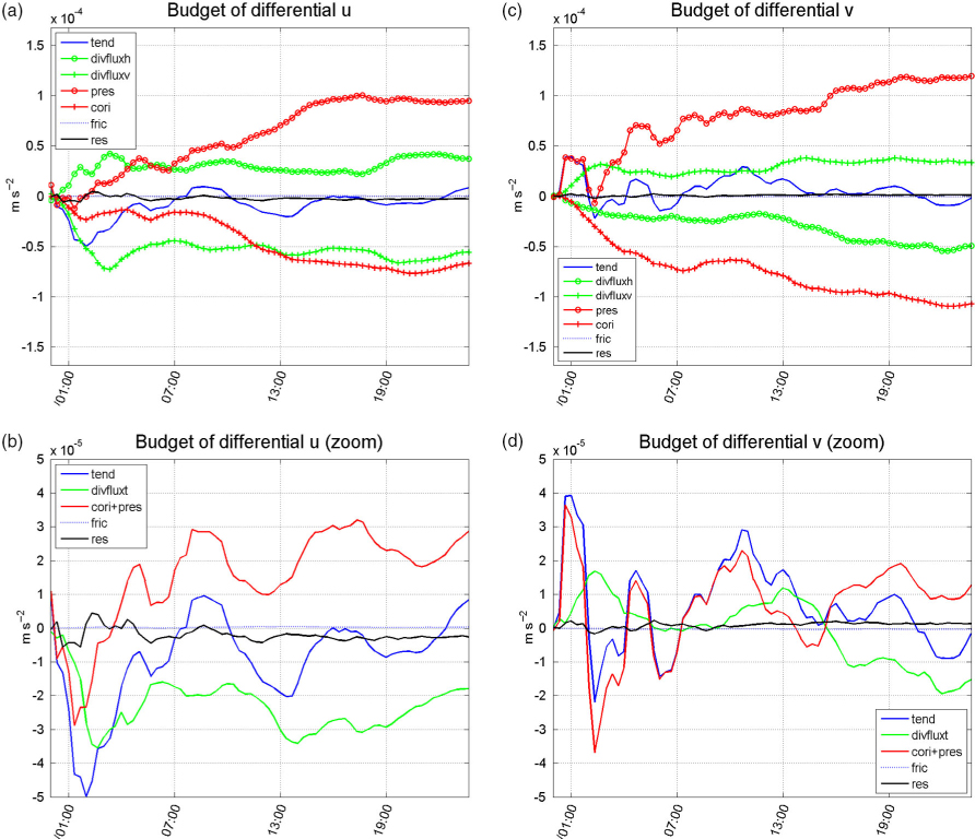
Fig. 13.
As in Fig. 10, except for the differential budget of KH. (a) tendency, (b) sum of the source terms, (c) pressure work, (d) total-flux divergence, (e) friction, (f) horizontal flux divergence, (g) residual term and (h) vertical flux divergence.
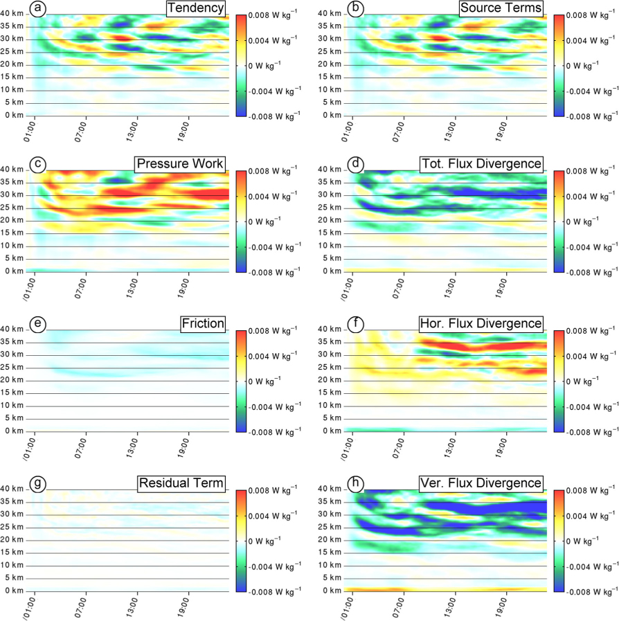
Fig. 14.
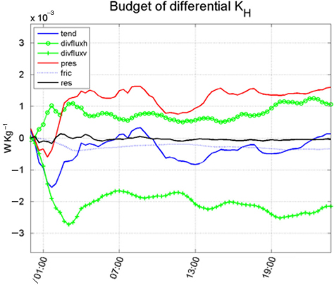
As in Fig. 8a, except for the terms of the budget of differential KH in W kg−1. The coefficients displayed are the tendency (solid blue line), the horizontal flux divergence (solid green line with circles), the vertical flux divergence (solid green line with plus signs), the pressure work (solid red line), the frictional dissipation (dashed dark line) and the residual term (solid dark line).