
1. Introduction
Long-term improvements in atmospheric general circulation models (GCMs) used in numerical weather prediction and climate simulations originate from gradually refined representations of atmospheric phenomena, especially of the subgrid-scale physical processes. In these models, the processes are represented by parameterisation schemes where the subgrid-scale variability is expressed using model variables of the resolved scales. Moreover, the schemes contain so-called closure parameters. The purpose of these model parameters is to encapsulate some atmospheric processes or properties which are not affordable for explicit modelling. The development process of the physical parameterisation schemes involves basically two steps: derivation of individual parameterisation schemes, and constraining of the schemes with large-scale observations (Lohmann et al., 2007). Here, large-scale observations means observations that are available for model tuning at the GCM scale. In the first step, dedicated laboratory measurements or focused field measurements campaigns are used, if a scheme cannot be derived from the first principles. The second step accounts for the fact that individual schemes are often valid for small scales, while in the context of GCMs, the schemes are applied in a relatively coarse resolution over a wide range of spatial and temporal scales. Thus, the schemes of interest have to be tuned such that the model indeed simulates the key atmospheric quantities within the uncertainty of some large-scale observational constraint. In practice, the closure (or, tuning) parameters provide the necessary degrees-of-freedom so that a realistic model response can be obtained.
In GCMs, a comprehensive set of physical parameterisation schemes are assembled together and embedded in the solver of the atmospheric dynamics. Time-space truncation and numerical approximations render, however, all model components to some extent imperfect. These model imperfections lead to systematic and random simulation errors. The systematic errors appear as a climate drift in the model simulations. The geographical patterns of these errors tend to develop very early in the simulation (Jung, 2005), and the so-called systematic initial tendency errors can be used for diagnosis and attribution of model errors to some particular atmospheric processes (Klinker and Sardeshmukh, 1992). In fact, there are attempts to estimate the initial tendency model errors and thus parameterise unrepresented physical phenomena in order to reduce systematic model errors (Kaas et al., 1999; D'Andrea and Vautard, 2000). Clearly, in the model simulations, there are multitudes of errors with different sources and the errors are in mutual non-linear interaction. Thus, it is not a surprise that it is very hard to improve the general model performance by improving the realism of representation of individual physical parameterisations (Jakob, 2010). Therefore, for a given model formulation, it is natural to strive towards optimal predictive skill by tuning the available degrees-of-freedom, that is, the closure parameter values. The estimation techniques range from trial-and-error to sophisticated parameter estimation techniques (e.g. Severijns and Hazeleger, 2005; Kunz et al., 2008; Järvinen et al., 2010; Neelin et al., 2010). The closure parameter values corresponding to the optimal predictive skill naturally depend on the level of approximation of the prediction system.
There is thus a dilemma on the uniqueness of weather and climate model closure parameters: one can either anchor the parameter values to the observable truth obtained, for example, via measurements from focused field campaigns, or tune the parameter values to account for the imperfections in the prediction system. It is qualitatively obvious that these two do not necessarily coincide and a practical optimum is a compromise between the two. In this article, we demonstrate that this dilemma exists. An outline of the demonstration is as follows. We use a low-order prediction system where synthetic observations are created using a modified version of the Lorenz-95 model (Lorenz, 1995; Wilks, 2005). As a prediction model, we use the standard Lorenz-95 model where the subgrid-scale effects on resolved scales are represented by a linear bulk parameterisation containing two closure parameters. Thus, the prediction model is imperfect. Data assimilation of the synthetic observations is performed using either extended Kalman filter (EKF) (Kalman, 1960) or ensemble adjustment Kalman filter (EAKF) (Anderson, 2001). We observe that the optimal prediction model corresponds to a unique but different parameter setting depending on the choice of the data assimilation component. The conclusion is that the dilemma exists.
Since the optimal closure parameter values depend on the implementation of the prediction system, such as the choice of the data assimilation algorithm, methodology for tuning the parameters specifically for each prediction system is needed. Here, we present such a method, using a combination of the so-called filter likelihood approach, where the likelihood is formulated based on the output of the filtering methods (Singer, 2002; Hakkarainen et al., 2012) and a Markov chain Monte Carlo algorithm (Haario et al., 2001, MCMC). We show that the approach yields parameter values that are close to the ones corresponding to optimal filter accuracy. In addition, we demonstrate how the approach can be implemented via the Data Assimilation Research Testbed software environment (Anderson et al., 2009, DART).
2. Methods and experimentation
In this section, an introduction to parameter estimation using the filter likelihood approach is given. It is then tested using the modified Lorenz-95 model.
2.1. On state estimation methods
One of the most common techniques for state estimation is Kalman filtering (Kalman, 1960). The basic idea in all filters is to obtain the posterior state estimate and some error statistics, typically the error covariance matrix , given the prior information and the observations y k at time step k.
The posterior state estimate can be transported to the next filtering time step to become the new prior state by using the forecast model. For the state vector, this is usually straightforward, but the fundamental question in filtering is how to transport the uncertainty in time. In EKF, this problem is solved by calculating the prior covariance matrix at time k as
where Q k is the model error covariance matrix and M k is the tangent-linear forecast model. If the dimension of the state space is high, such as in large-scale atmospheric models, eq. (1) becomes impossible to compute without approximations.
One approximative approach is ensemble filtering, where the uncertainty is transported to the next filtering time step by transporting an ensemble of states using the forecast model. The difficulty (and variety) of the ensemble methods lies in how to update the prior ensemble in the analysis step. There are many alternatives, for instance the ensemble adjustment Kalman filter (Anderson, 2001, 2010), which belongs to the family of the so-called ensemble square root filters (Tippett et al., 2003). In this study, the EAKF was chosen because it is a deterministic ensemble based filter, that is, it does not include randomisation of the ensembles. The non-randomness is important, since in Section 2.3 we want to create a likelihood function based on the filtering outputs and the randomness in the likelihood would complicate the parameter inference (Dowd, 2011; Hakkarainen et al., 2012). Also, EAKF was chosen because it is conveniently available in the data assimilation research testbed (Anderson et al., 2009, DART) and widely applied (e.g. Schwartz et al., 2011; Torn and Davis, 2012).
In EKF, the modelling errors of the forecast model are taken into account via the error covariance matrix Q k . In EAKF (and in ensemble square root filtering in general), the neglect of unknown model errors can lead to over-confidence in the prior state and hence ignorance of the observations in the analysis, which can lead to filter divergence. This is effectively circumvented by introducing covariance inflation factors (Anderson and Anderson, 1999). In addition, the sampling errors related to the limited ensemble size (undersampling), are mostly removed by localisation (Hamill et al., 2001), where observations affect only nearby grid points.
2.2. On parameter estimation
Parameter estimation techniques developed for the atmospheric models can be divided in two categories: online and offline methods. In online methods, it is assumed that model parameters are not static quantities, but can evolve adaptively, for example, as a part of a state estimation process (e.g. Annan et al., 2005) and are thus computationally relatively cheap to implement. Typically, a statistical interpretation is lacking in online methods, since the rate of change of the parameters is controlled by the user. In this article, these online methods are not discussed further. Instead we use offline methodology, where a predetermined (training) set of observations y is used for tuning the parameter values.
In Bayesian methodology (e.g. Gelman et al., 2003), the knowledge about the unknown parameters is inferred from the posterior distribution:
which is evaluated using the prior p(θ) and the likelihood p(y|θ). The prior contains the information that we have about the parameters based on the accumulated information from the past. The likelihood function specifies how plausible the observed data are given model parameter values. Therefore, defining a proper likelihood function is the central question in parameter estimation.
The parameter estimation problem is often written in a (cost) functional form with parameters as arguments. Different numerical methods can be used for optimising the cost function and point estimates, such as the Maximum a Posteriori (MAP) estimate, can be obtained. In addition, Monte Carlo methods like MCMC can be used for producing samples from the posterior distribution instead of a single point estimate, and studying the uncertainty in the parameter values. For large-scale applications, applying MCMC is challenging, since the methods can involve thousands of repeated likelihood evaluations, but ways to improve the efficiency of MCMC for high-CPU models have been recently developed (Solonen et al., 2012).
2.3. Likelihood via filtering methods
In this section, the filter likelihood concept is discussed in the context of the extended Kalman filter and the ensemble adjustment Kalman filter. The approach is known in the parameter estimation of stochastic models (e.g. Singer, 2002), but less studied in connection with deterministic, chaotic systems (Hakkarainen et al., 2012). For the sake of completeness, the derivation of the likelihood computation is briefly reviewed in the Appendix.
When EKF is considered, the filter likelihood formula, i.e., the likelihood for observing y 1:n given the parameters θ, can be written as
where is the innovation vector and is its error covariance matrix at time k. Operator denotes the matrix determinant. In filtering, is the observation operator that maps from the state space to the observation space and H is its linearization. The prior state is given by the model, the prior covariance matrix is given by the Kalman filtering formulas [eq. (1)] and R k is the observation error covariance matrix.
Essentially, the filter likelihood formula [eq. (3)] depends on the summation over the cost functions J k , where the normalising term has to be accounted for, because it implicitly depends on the parameters θ. The dependence comes from eq. (1) via the tangent-linear forecast model. It should be noted that eq. (3) itself does not require that and its covariance matrix are calculated using EKF. In principle, any state estimation method that produces these prior estimates could be used.
In EAKF, as implemented in the DART system, the discrepancy between the prior ensemble and the observations are calculated in the observation space for every single observation sequentially. The update of the ensemble and the weights are also calculated sequentially in the observation space. Thus, it is natural to adopt this approach also in the filter likelihood calculations. The cost function part of the filter likelihood formula [eq. (3)] can be calculated sequentially as a sum
where y l is an individual observation and is the individual prior ensemble mean in observation space and and are their variances, respectively. The prior ensemble mean depends implicitly on y l−1, because of the sequential update. The summation goes through all the individual observations y 1:L,k at time k. The DART system does not provide the above computation, but including these in the DART code can be easily implemented.
2.4. Model and data
To explore the filter likelihood calculation, a modified version of the Lorenz-95 system is used (Lorenz, 1995; Wilks, 2005). The full system consists of two interrelated variables X and Y, and it is written as
where i=1,…, I and j=1,…, JI. That is, each of the ‘slow’ state variables X i are forced by a sum of the additional fast variables Y j . The fast variables have dynamics similar to the slow variables, but they are also coupled with the slow variables. In the model, cyclic boundary conditions, i.e., X I+1=X 1 and Y JI+1=Y 1, are used. In this paper, values I=40, J=8, F=F Y =10, h=1 and c=b=10, adopted from Leutbecher (2010), are used.
The parametrized forecast model for the full system reads
where is the parameterization in which the effect of the missing ‘sub-grid’ scale fast variables Y j are modeled using only the single, ‘resolved’, local variable X i .
The aim of the experiment is to tune the parameters θ=(θ 0, θ 1) given a synthetic set of observations y 1:n , computed by the full set of equations in (5) and (6) with additive noise, using the filter likelihood technique. In the experiment, one filtering step (‘24 h’) is 8 model integration steps (‘3 h’). Here the number of assimilation steps n=100 (‘days’), and hence during each run the model is integrated 100×8 times. The experiment is adopted from Hakkarainen et al. (2012) and a more comprehensive introduction is given there.
2.5. Experiment setup
In the experiment, the parameter values are sampled from the posterior distribution {consisting of filter likelihood [eq. (3)] and uninformative prior} using an adaptive Metropolis algorithm (Haario et al., 2001). The chain length is selected to be 3000 and the first 500 samples (the burn-in period) are discarded. The filter likelihood MCMC experimentation is synthesised with the following pseudo-algorithm, where the superscript m on θ denotes MCMC chain index:
Step 0:
Initialise the MCMC run and select θ 1.
Step 1:
Propose a new candidate for the parameters.
Step 2:
Run the state estimation system using and evaluate formula [eq. (3)] during the run.
Step 3:
Accept with probability .
Step 4:
If is accepted set , else set .
Step 5:
Set m=m+1 and go to step 1 until m is equal to the chain length.
In our implementation, we use an uninformative (flat) prior, which means that the prior is a constant, p(θ) α1. Then, the prior term cancels out in Step 3 of the above algorithm, since .
For readers not familiar with MCMC, a short introduction is in order. The MCMC algorithm works by generating candidate values from a proposal distribution, which in our case is Gaussian centred at the current parameter value. The candidates are then either accepted or rejected according to a simple rule that contains the ratio of the posterior densities at the proposed point and at the current point, see Step 3 of the above algorithm. One can see that moves ‘upward’ (to a point with higher posterior density) are always accepted. However, also moves downward can be accepted, and the resulting random walk ends up exploring the posterior distribution without converging to a single point. The algorithm is a standard tool in statistical analysis and can be shown to yield samples from the correct target density. Here, we apply an adaptive version of the algorithm Haario et al. (2001), where the proposal distribution is automatically tuned to better match the posterior distribution. For more details on MCMC, see Robert and Casella (2005).
Using the filter likelihood [eq. (3)] for MCMC, we are able to estimate both the model parameters θ and the filter-specific tuning parameters. In the experiments, for the EKF version, the model error covariance matrix is parameterised as follows
where I is an identity matrix. The parameter λ is tuned together with the model parameters θ 1 and θ 1. In the EAKF version of the filter likelihood, the prior covariance inflation factor and the cut-off radius related to localisation (Gaspari and Cohn, 1999), defined in the DART setup, are tuned together with the model parameters θ.
As a validation metric for the parameters, we use the average root mean squared error (RMSE) defined as
where is the true state and is the posterior estimate. We evaluate RMSE on a fixed grid for θ 1 and θ 2 keeping the filter-specific parameters fixed.
2.6. Results
The experiments are started by a step, where all parameters (i.e. filter parameters and the model parameters) are estimated together with MCMC. In Fig. 1, pairwise MCMC samples using EKF (left panel) and EAKF (right panel) are shown. It can be seen, that the marginal distributions are rather Gaussian and all parameters are identified. Based on the mean values of the MCMC chains, values −4.8824, 1.4310 and 0.1889 were chosen for λ, the prior inflation factor and the cut-off radius, respectively.
In the second step, to further underline the difference in the model parameter estimates in the usual situation where the filter parameters are fixed, we calculate the conditional θ distributions using MCMC by fixing the filter parameters to the mean values found in the previous step. For the validation purposes, the RMS error [eq. (9)] is evaluated on a fixed grid to explore the parameter space for ‘all’ possible pairs of θ 0 and θ 1.
The results are illustrated in Fig. 2, where the 50% and 95% probability contours calculated from the EKF and EAKF MCMC chains are plotted using solid and dashed lines, respectively. The colours on the background indicate the average RMSE values [eq. (9)] for EKF (left panel) and EAKF (right panel). We observe that the closure parameter values that correspond to the lowest average RMSE values for EKF and EAKF are not the same. This implies that the optimal parameter values for EKF are not optimal for EAKF and vice versa. This shows that there is a dilemma of the uniqueness of the model closure parameters: an identical model formulation can have more than one optimal parameter value combination. This can be explained by the fact that the two data assimilation components have different systematic approximation errors, and these errors are compensated, to some extent, by the different parameter values in the forecast model. In this sense, the forecast model parameter values should be considered as filter-dependent quantities. The consequences of this result are discussed below in Section 3.
Figure 2 also depicts that the filter likelihood method captures the optimal parameter values correctly: the lowest posterior RMSE values are close to the obtained posterior distributions. In addition, it can be seen that the results produced by the EKF and EAKF versions of the filter likelihood technique are similar, but not identical. The posterior distribution obtained using EKF is closer to the parameter values that yield low RMS error for EKF. And vice versa: the parameters estimated using EAKF are closer to the optimal values for EAKF than the ones obtained by EKF. That is, applying the filter likelihood technique seems to provide rather good filter-specific parameter estimates. In this study, the RMSE values produced by EKF are lower than those produced by EAKF (see the RMSE values at the background of Fig. 2), which was expected. In addition, it can be noted, that the choice of data assimilation component has a much larger effect on the RMSE than the exact values of the model parameters.
3. Discussion and conclusions
In this article, we presented a numerical experiment with the purpose to simulate the prediction model parameter estimation problem in chaotic systems. We studied a simplified prediction system, which consists of a modified Lorenz-95 system as the prediction model, where the net effect of fast variables is represented by a two-parameter linear scheme. Two versions of the Kalman filter were used as different data assimilation components. We have shown that depending on the version of data assimilation that is applied, either the extended Kalman filter or the ensemble adjustment Kalman filter, the optimal prediction model tuning parameters corresponding to the highest system accuracy have two distinct optima. Accuracy is measured here as the RMS errors of the state estimate against the known truth. Replacement of EKF with EAKF implies a major change to the prediction system and it is only natural that the prediction model parameters need re-tuning.
In addition, we have demonstrated a method that can be used to estimate the closure parameters for each prediction system component separately. The approach is based on computing the likelihood using the output of the data assimilation system. We also demonstrate how Markov chain Monte Carlo sampling methods can be used on top of this likelihood formulation. The method recovers the optimal forecast model parameter values for both data assimilation systems. In addition, both the forecast model parameters and the data assimilation related parameters can be estimated. In our case, the data assimilation related parameters were the model error covariance matrix in EKF, and covariance inflation and localisation parameters in EAKF.
The models applied in operational weather forecasting are far more complex than the system applied here. If we assume that the behaviour discovered here scales up, it has some consequences for tuning of large-scale systems. Traditionally, model releases are carefully fine-tuned and parallel tested associated with forecast model changes. Changes in data assimilation are, however, typically considered independent of forecast model fine-tuning. According to the result presented here, this should not be the case. If the data assimilation component undergoes a major revision but the prediction model remains the same, then the prediction model tuning corresponds to the previous version of the data assimilation component and may thus be suboptimal. In this case, the correct procedure would be to consider model tuning, too.
Finally, this work considered a low-order prediction system. Our future work will be directed towards quantifying how this result scales-up to more realistic systems. We will use the ECHAM6 prediction model together with the DART toolbox to study this question.
4. Acknowledgements
We would like to acknowledge the National Center for Atmospheric Research for making the Data Assimilation Research Testbed available on-line. The research has been financially supported by the Academy of Finland (project numbers 127210, 132808, 133142, 134935 and 134999) and the Centre of Excellence in Inverse Problems Research. Additionally, this work was funded by the European Commission's 7th Framework Programme, under Grant Agreement number 282672, EMBRACE project, and the Nessling Foundation.
Appendices
5. Appendix
A.1. Derivation of the filter likelihood formula
We present the derivation of the filter likelihood formula [eq. (3)], briefly. A more comprehensive discussion is given in Hakkarainen et al. (2012).
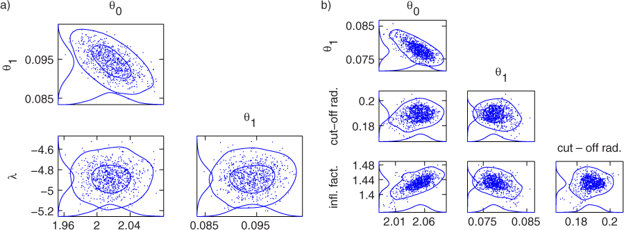
Fig. 1
Pairwise MCMC samples using EKF (left panel) and EAKF (right panel) version of the filter likelihood formula [eq. (3)]. In addition to the model parameters θ 0 and θ 1, filter related parameters are sampled too. Contours illustrate 95% and 50% probability regions. Also, the one-dimensional marginal densities are illustrated.
Let us consider the following general state space model.
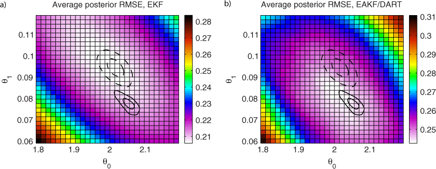
Fig. 2
Average posterior RMSE values [eq. (9)] when using EKF (left panel) and EAKF (right panel). Lower values indicate better performance. Solid and dashed lines indicate the 50% and 95% probability regions as obtained with MCMC in case of EAKF and EKF, respectively. RMSE values are depicted by the background colour scheme. Note the difference in colour scales.
of state x k , observations y k and parameters θ, respectively. Our goal is to find the posterior distribution . In filtering, the previous state estimate can be transported to the next time step's prior by using the prediction model
and in the analysis step the prior is updated by y k using the Bayes’ formula
The predictive distribution for next observations can be obtained by
Using Bayes’ formula and the chain rule we obtain
where can be calculated using eq. (A6).
In extended Kalman filtering the predictive distribution is
Now, applying this to eq. (A8) we can obtain eq. (3).