
Table 1
Observation types assimilated in the experiment
[i] The third to sixth columns show the average number of observations assimilated on each vertical layer in one analysis (in thousands). Peak pressure of weighting function is used as vertical position of satellite radiance observation. u, v, T, q and Ps represents u and v wind components, temperature, specific humidity and surface pressure, respectively.
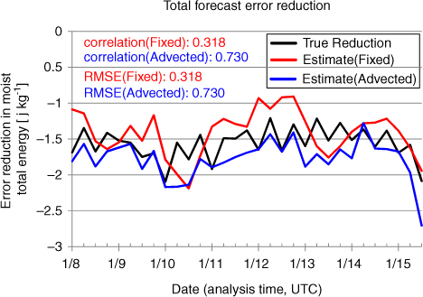
Fig. 1
Time series of the total forecast error reduction of each estimate (unit: J kg−1). Black, red and blue lines show the actual forecast error reduction verified against the own analysis, estimated error reduction from the EnKF-based method with fixed localisation (fixed) and with moving localisation (advected). Numbers on upper left corner show the correlation and RMSE of each estimate to the actual forecast error reduction.
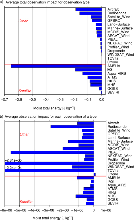
Fig. 2
Estimated average 24-hour forecast error reduction contributed from each observation types (moist total energy, J kg−1). (a) represents the total error reduction and (b) represents error reduction per observation.
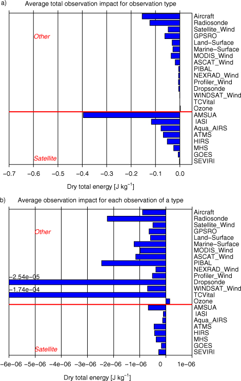
Fig. 3
Same as Fig. 2 but with the dry total energy norm (J kg−1)
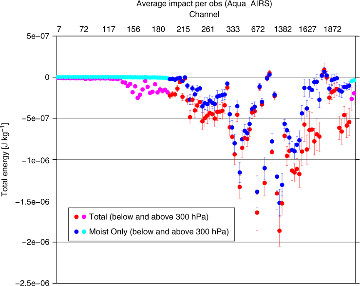
Fig. 4
Estimated AIRS satellite radiance observation impacts classified by channel with the moist total energy (red for channels sensitive below 300 hPa and magenta above 300 hPa, J kg−1), and only the moist term of the total energy (blue for channels sensitive below 300 hPa and aqua above 300 hPa, J kg−1). Average estimated forecast error reduction from a single observation is shown. Vertical bars represent the 95% confidence interval of the average values.
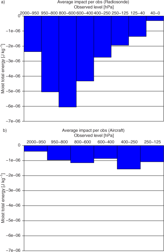
Fig. 5
Estimated average observation impacts of a) radiosonde and b) aircraft classified by observed level (moist total energy, J kg−1). Average estimated forecast error reduction by a single observation is shown.
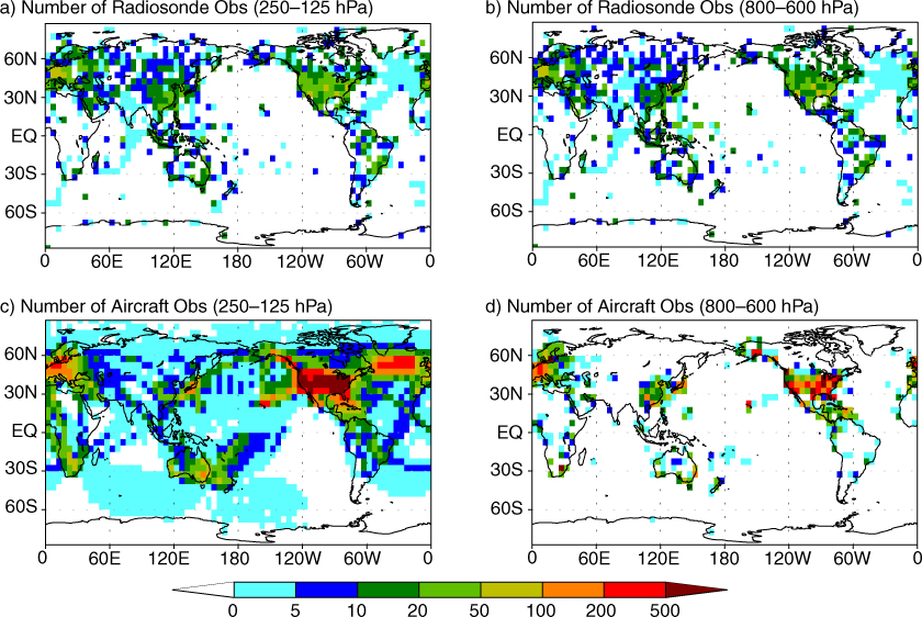
Fig. 6
Average number of assimilated radiosonde observations (a) from 250 to 125 hPa, (b) from 800 to 600 hPa and aircraft observations (c) from 250 to 125 hPa and (d) from 800 to 600 hPa in each 5°×5° area for one analysis.
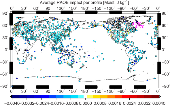
Fig. 7
Average impact (moist total energy, J kg−1) of a single radiosonde profile from the fixed land stations. Only the stations that have more than 20 profiles in the period are shown. Numbers 4220 (Egedesminde) and 4270 (Narssassuaq) indicate the location of the stations shown in Fig. 8.
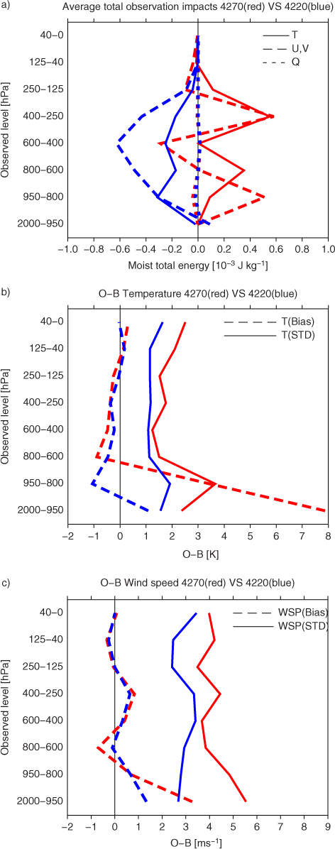
Fig. 8
Comparison of the radiosonde observations from Narssassuaq (red line, 4270) and Egedesminde (blue line, 4220) showing (a) average impacts (J kg−1) of each observation element (solid: temperature, dashed: winds, dotted: humidity) on each pressure level by one profile and observation departure statistics (dashed: bias, solid: standard deviation) of (b) temperature (K) and (c) wind speed (m s−1).
Table 2
Width of longitude used for the local area on each latitude band
Table 3
List of local 24-hour forecast failure cases (initial time from 00 UTC, 8 January 2012, to 18 UTC 7 February 2012)
[i] The third, fourth and fifth columns show the forecast error size normalized with the time-averaged error, the rate of the error size compared with the error of 30-hour forecast from the previous analysis, and the number of areas that meet the criteria. Sixth column shows the denied observation type based on the observation impact estimates, number of denied observations and total number of observations with this observation type assimilated in the original analysis. Finally, seventh column shows the change of the 24-hour local forecast error for observation denial experiment and corresponding estimated forecast error change in the parenthesis. The case shown in bold font is the example shown in Fig. 9.
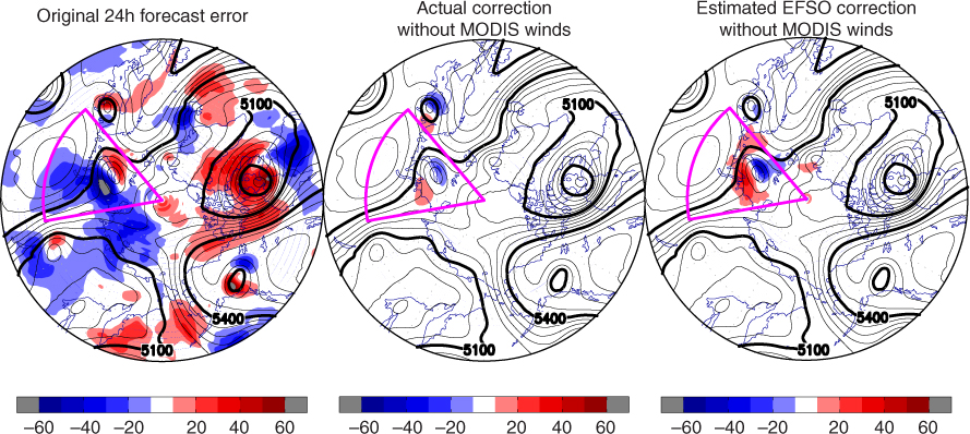
Fig. 9
Twenty-four hour forecast error of 500 hPa geopotential height (unit: m, 18 UTC 6 February 2012 initial) from original analysis (left) and forecast change due to the removal of the MODIS polar wind observations in the data-denial experiment (middle: actual change and right: projection on the ensemble perturbations). Black contours show the analysis. Magenta cones show the target area of the observation impact estimate.