
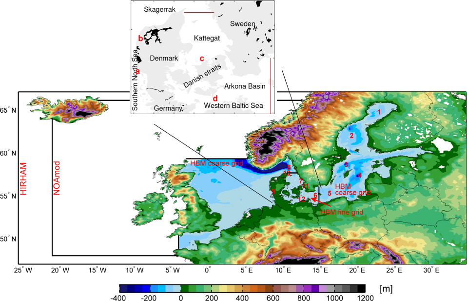
Fig. 1
Topography of model areas: HIRHAM – the regional atmospheric model covering the entire area; NOAmod – the surge model covering the northeast Atlantic Ocean and the North Sea (NS), enclosed by the black lines; HBM coarse grid – the regional ocean model covering the North Sea, with open boundaries at 59.25°N and 4.08°W, and the Baltic Sea; and HBM fine grid – the transition zone including the Kattegat, the Danish straits and the Arkona Basin (AB) (indicated in the inset figure), two-way nested with the outer model. Details of model grids are listed in Table 1. Positions for SST stations are indicated by numbers: 1, Bothnian Bay; 2, Bothnian Sea; 3, Landsort; 4, East Gotland Basin; 5, Bornholm Basin; 6, Arkona; 7, Kattegat; and 8, Skagerrak. Positions for tide gauges are indicated by numbers: 9, Esbjerg; 10, Hirtshals; 11, Hornbæk; and 12, Gedser. Positions for land wind stations are indicated in the inset figure by a, Blåvandshuk; b, Thyborøn; c, Gniben; and d, Gedser. Stations coordinates are listed in Table 2.
Table 1
Regional atmosphere and ocean model grids
Table 2
Station list (locations are indicated in Fig. 1)
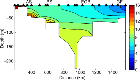
Fig. 2
Depth profile of the Baltic Sea from the Sound via the Arkona Basin (AB) and the Bornholm Sea (BS) to the Eastern Gotland Basin (EGB) and the Gulf of Finland (GF), showing the average salinity stratification from the standard simulation (1990–2010). Positions of the stations are indicated in Fig. 7.
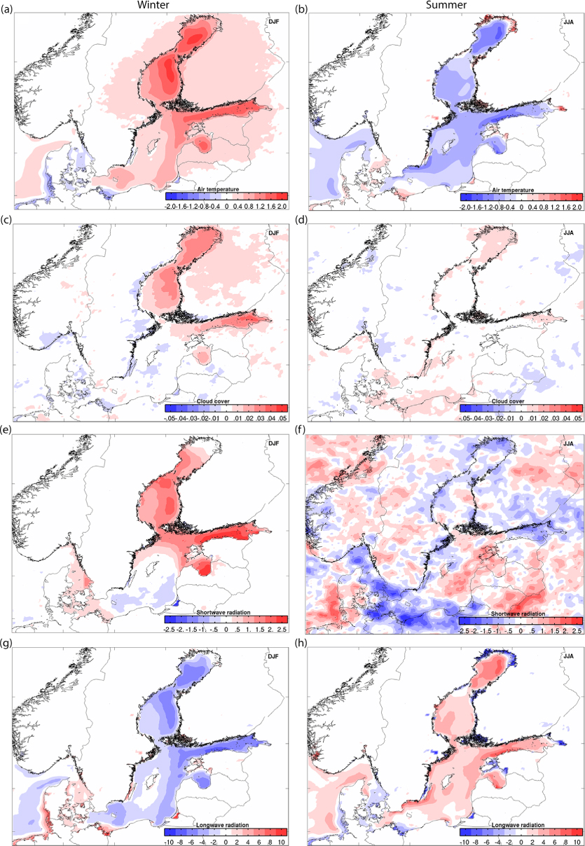
Fig. 3
Differences in seasonal mean (1990–2010) between the coupled and standard simulation for surface variables: 2 m air temperature in °C (a and b), cloud cover (c and d), net incoming shortwave radiation in W m−2 (e and f) and net incoming longwave radiation in W m−2 (g and h). The left and right panels are winter (December through February, or DJF) and summer (June through August, or JJA) means, respectively.
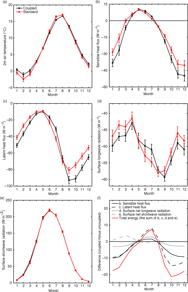
Fig. 4
Monthly means (1990–2010) with error bars for the field average over the Baltic Sea (sea points within 54–66°N, 15–30°E) for (a) 2 m air temperature; (b) sensible heat flux; (c) latent heat flux; (d) surface net longwave radiation and (e) surface net shortwave radiation, all compared for the coupled (black) and standard (red) simulation; and (f) flux differences (coupled minus prescribed simulation) for (b), (c), (d), (e) and total energy (i.e. the sum of (b)–(e)). Error bar indicates one standard error of the mean over the 21 yr. Overlap of error bars indicates that the two simulations are not significantly different.
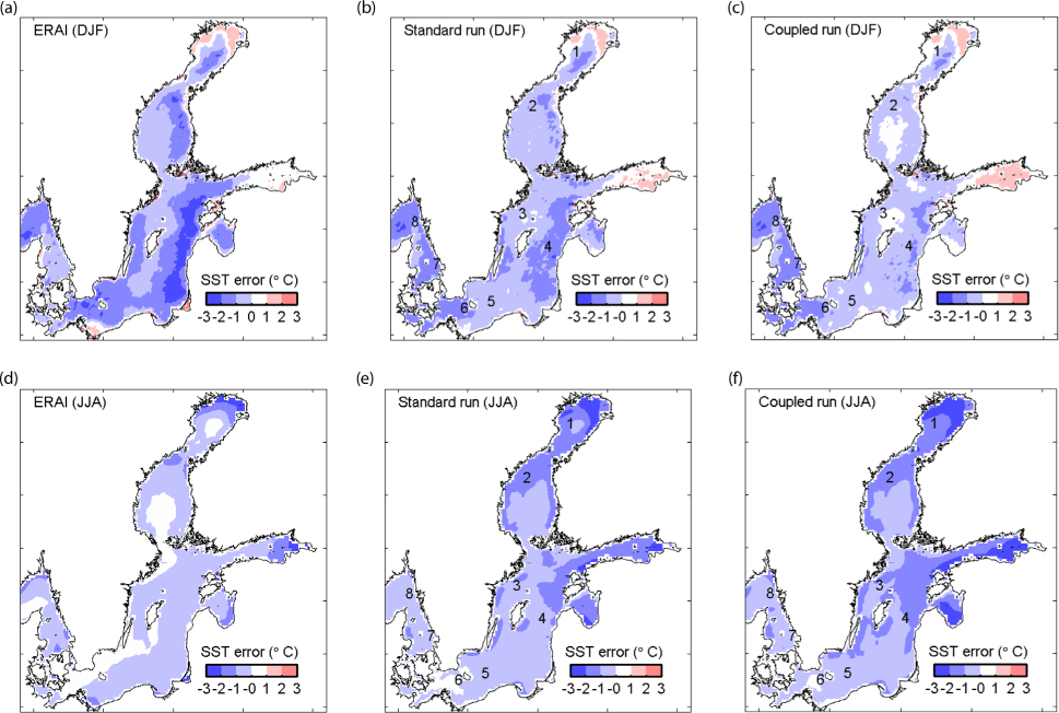
Fig. 5
Differences in seasonal mean SSTs (1990–2010) relative to satellite data. Winter (DJF) and summer (JJA) means are presented on the top and bottom panels, respectively. The results from ERAI reanalysis and from the standard and coupled run are shown from left to right, respectively. Sea ice is assumed when missing values occur in DJF in the satellite data. SST is set to the approximate freezing point of −0.3°C where ice covered. The numbers indicate the station indices defined in Fig. 1 and Table 2 which highlight the spatial differences in model errors.
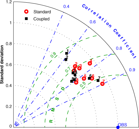
Fig. 6
Taylor diagram assessing the deseasonalised time series of SST in two simulations with correlation coefficients, normalised standard deviations and RMSDs to in situ observation (OBS). The time series from 2000 to 2010 are chosen at eight selected stations. The nearest model grid points are used, and the results are extracted according to the date of measurements. The numbers indicate the station indices defined in Fig. 5 and Table 2. The results from the coupled and standard run are indicated by black solid squares and red open circles, respectively.
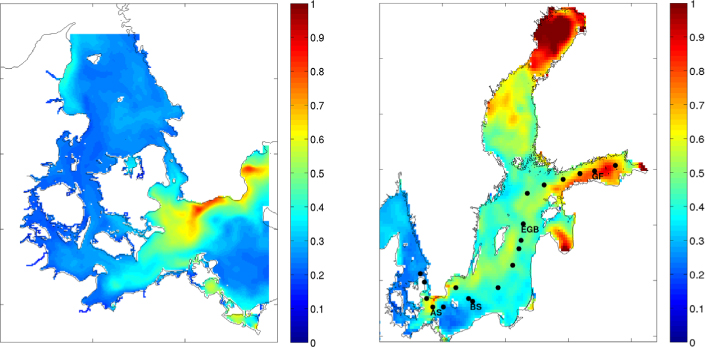
Fig. 7
RMS differences of the JJA monthly mean SST between the coupled and standard simulation in the period 1990–2010. Positions of the stations from the southwest to northeast Baltic Sea, at which a depth profile of average salinity is shown in Fig. 2.
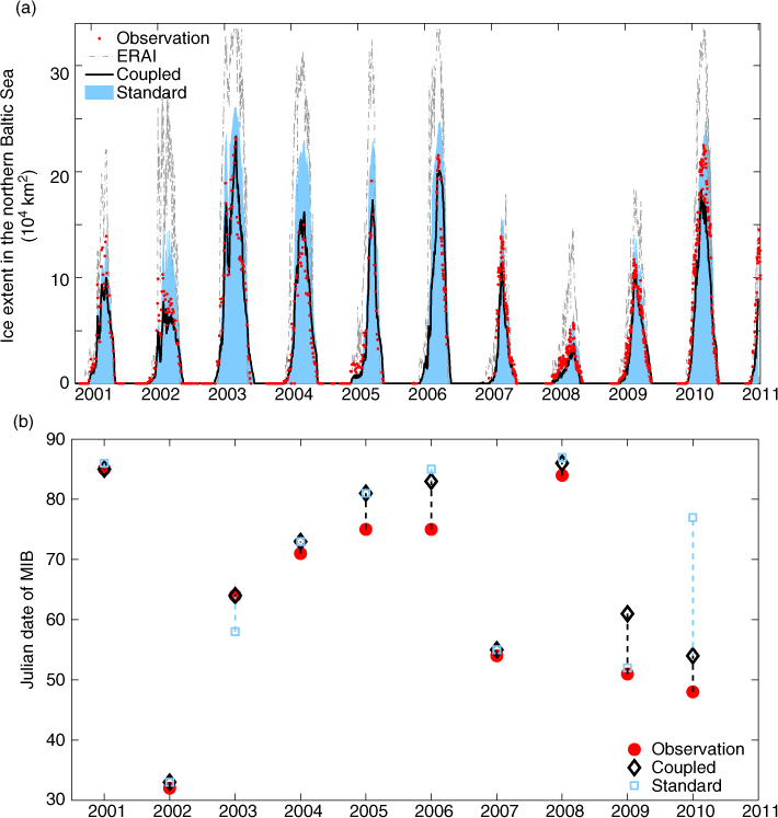
Fig. 8
(a) Daily ice extent from observations (red dots), ERAI reanalysis (grey line) and the coupled (black line) and standard (shaded area) simulations in the northern Baltic Sea (58.0–65.8°N, 17.17–30.17°E) since 30 October 2000. (b) Julian date of annual maximum ice extent (MIB) of the whole Baltic Sea from observations (red) together with the coupled (black) and standard (blue) simulations. The dashed lines between modelled and observed dates indicate the length of the lag time.
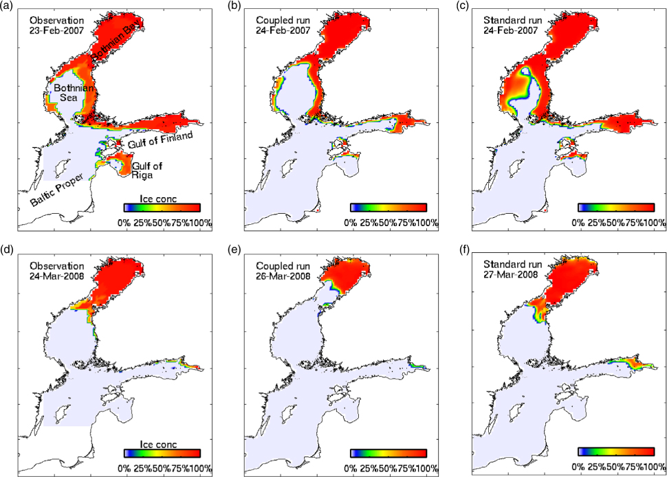
Fig. 9
Observed and modelled ice concentration distributions for the dates of MIB in the Baltic Sea in 2007 (top panels: (a)–(c)) and 2008 (bottom panels: (d)–(f)) as defined in Fig. 8. Winters 2007 and 2008 are taken as examples of an average and an extremely mild winter according to the classification by Seinä and Palosuo (1996).
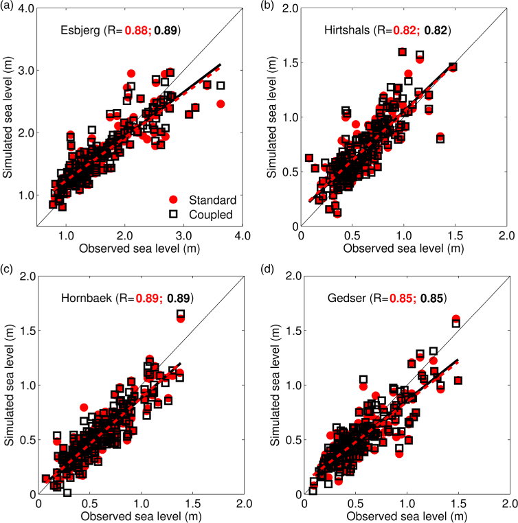
Fig. 10
Scatterplots of monthly maxima of hourly sea levels at Esbjerg, Hirtshals, Hornbæk and Gedser. Observations are plotted on the x-axis, which are retrieved from DMI tide gauges. Model results are plotted on the y-axis, indicated by black open squares (coupled) and red solid circles (standard). The correlation coefficients (R), with p<0.001, are given for both runs.
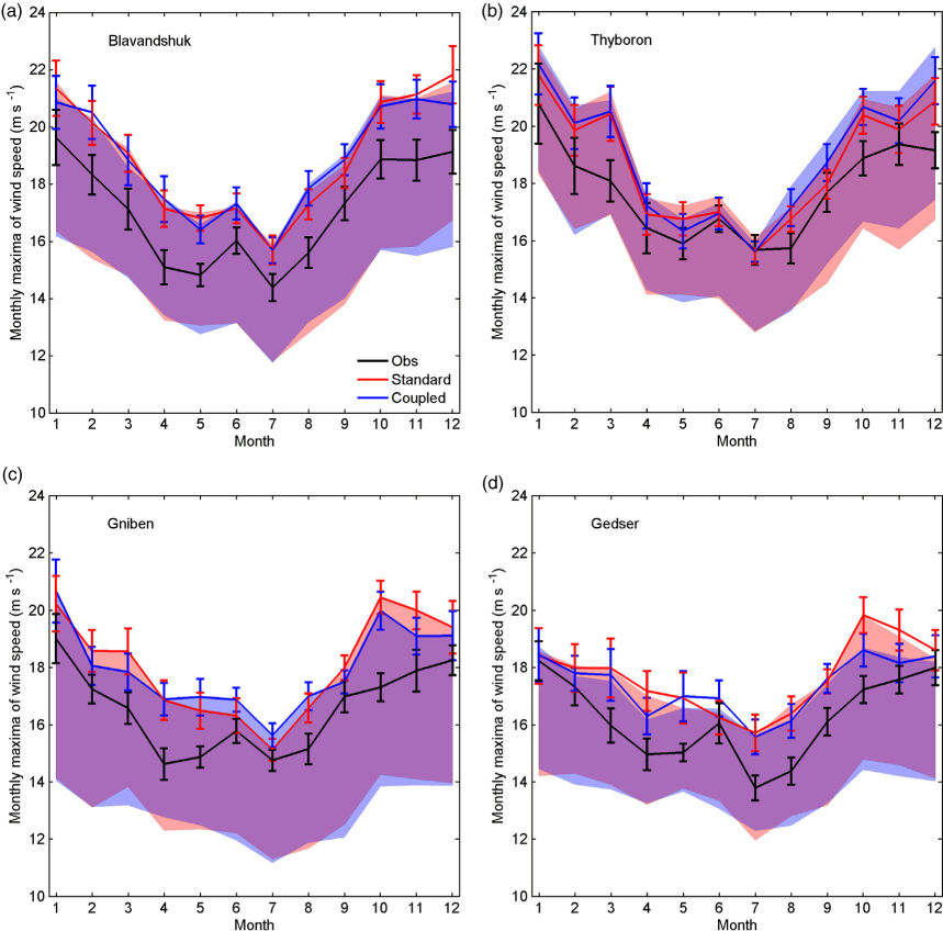
Fig. 11
Monthly mean maximum wind speeds (1990–2010) with error bars at Blåvandshuk, Thyborøn, Gniben and Gedser. The observations (black) are derived from continuous 10-min average readings at the DMI land stations. The modelled wind speed is taken from hourly instantaneous values at model grid points with land–sea fractions closest to the observation stations in the coupled (blue) and standard (red) simulations. Error bar indicates one standard error of the mean. The shaded areas show the model results from the sea grid (upper limit) and from the land grid (lower limit) closest to the observation stations.