Fig. 1.
The background wind vector, the observation wind vector, the analysis wind vector obtained by asm_uv (assimilating u and v) and the analysis wind vector obtained by asm_sd (assimilating sp and dir). For this illustration, we assume u,v, dir and sp can be analysed independently and B/R=1.
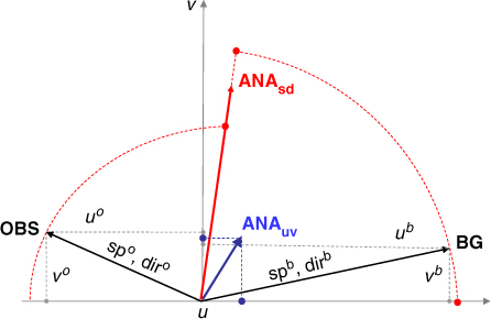
Fig. 2.
The ratio of asm_uv analysis wind speed to asm_sd analysis wind speed as a function of u o and v o , which is computed using eq. (15). The background wind vector (u b , v b ) is also shown.
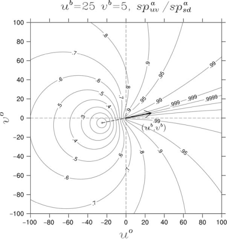
Fig. 3.
The background wind vector, the observation wind vector, the analysis wind vector obtained by asm_uv (assimilating u and v) and the analysis wind vector obtained by asm_sd (assimilating sp and dir). WRFDA is used with the default option (asm_uv) and with the new option (asm_sd).
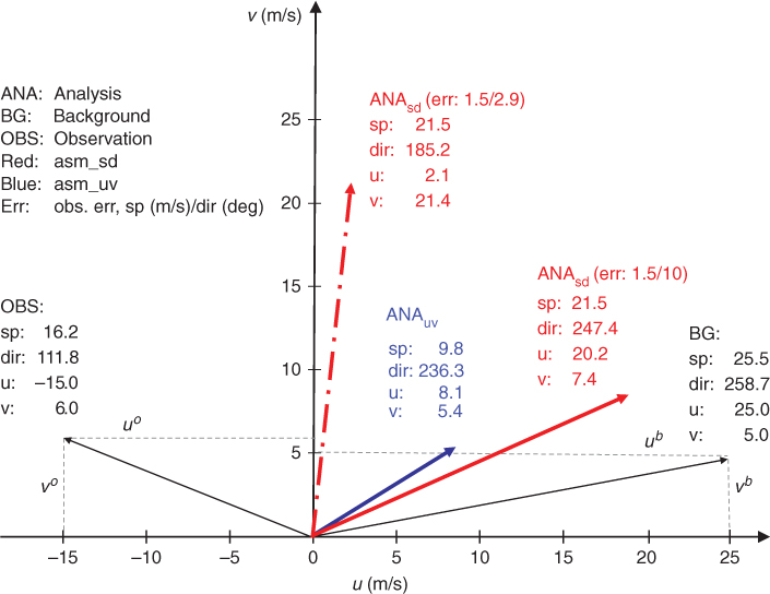
Fig. 4.
The ratio of asm_uv analysis wind speed to asm_sd analysis wind speed as a function of u o and v o , which is computed using WRFDA. The background wind vector, (u b , v b ), is also shown.
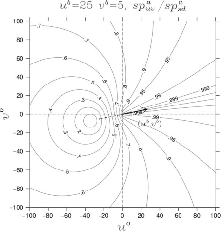
Fig. 5.
The wind analysis increments due to a single wind observation pair (−15.0 m s−1, 6.0 m s−1) or (16.2 m s−1, 111.8°) by asm_uv (left; a, c, e) and by asm_sd (right; b, d, f). The top two panels (a, b) are for u, middle two (c, d) for v and the bottom two (e, f) are for wind vectors (u,v). The observation location is indicated by a red dot. The analysis increment vector at the observation location is highlighted with a red vector.
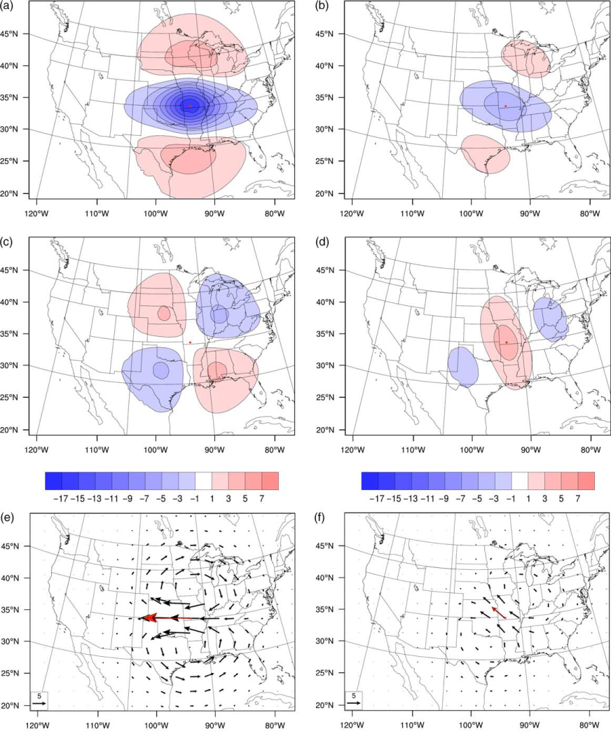
Fig. 6.
The 500-hPa geopotential height, winds and temperature of the reference atmosphere (i.e. the nature run) (a) and the FNL analysis (b), valid 0000 UTC 18 December 2011.
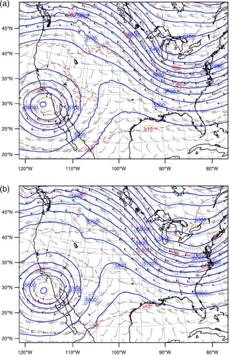
Fig. 7.
The model domain with horizontal distribution of simulated observations (dots) in the upper panel and an enlarged view of the small box in the upper panel with ‘nature run’ model grid points (dots), ‘assimilation run’ model grid points (crosses) and observation locations (large dots) in the lower panel.
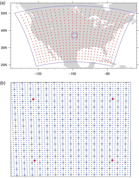
Fig. 8.
(a) Observation error variances, (δu o )2, (δv o )2, (δsp o )2 and (δdir o )2, which are computed by comparing the simulated observations against the direct respective variables within the reference atmosphere. (b) Observation error variances, (δu o )2 and (δv o )2, computed from (δsp o )2 and (δdir o )2 using eq. (16) and eq. (17). The contributions from (δsp o )2 only (labelled _sp) and from (δdir o )2 only (labelled _dir) are also shown.
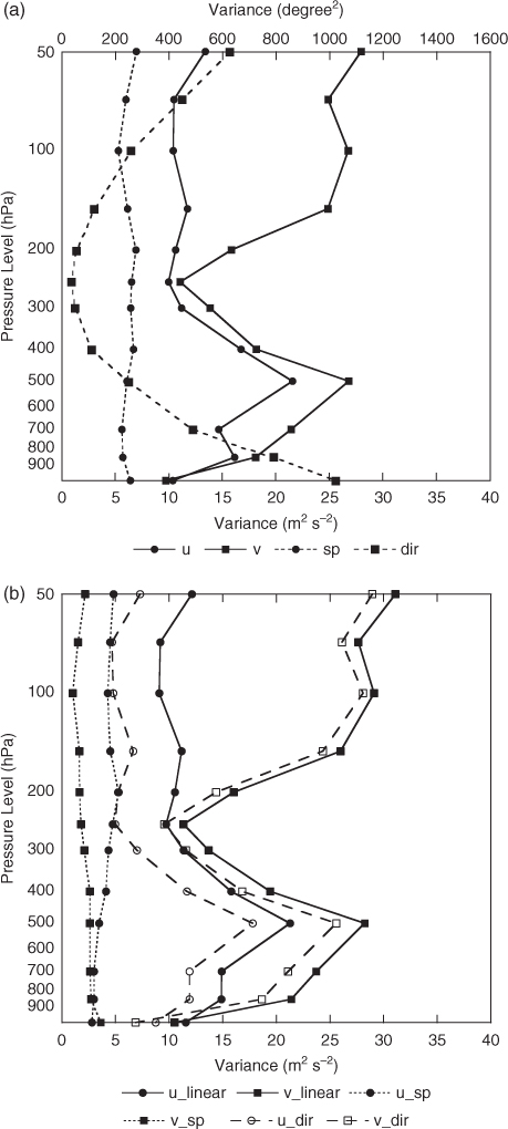
Fig. 9.
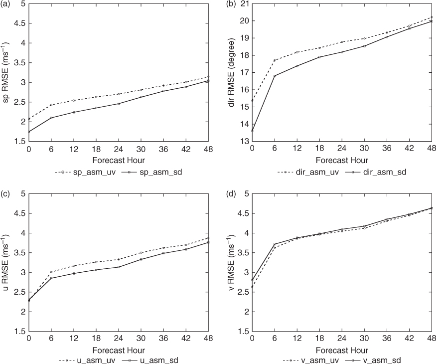
Time series of the average RMSE of nine cycles of 48-h forecasts, where sp and dir observation error is generated and then converted to u and v observation errors. The verification includes the four variables: sp (a), dir (b), u (c) and v (d).