
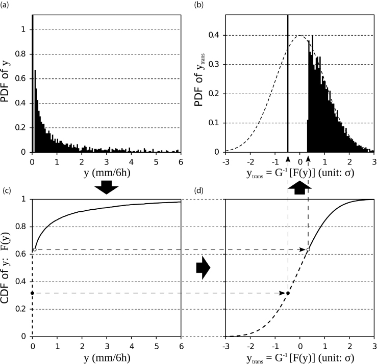
Fig. 1
The PDF and CDF of (a, c) the original precipitation and (b, d) the transformed precipitation at a grid point near Maryland (38.967°N, 78.75°W) in winter season (December–February) based on the 10-yr nature run. The procedure of the GT is from (a) to (c), to (d), and to (b) as indicated by the arrows.
PDF = probability density function; CDF = cumulative distribution function; GT = Gaussian transformation.
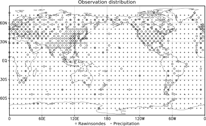
Fig. 2
The spatial distribution of conventional rawinsonde observations (open circle) and global precipitation observations (plus sign) used in the OSSEs.
OSSE = observing system simulation experiments.
Table 1
The observation errors for the simulated observations
Table 2
Design of all experiments
Experiment Raobs. Prcp. Gaussian transf.Criteria for prcp. assimilationObs. error of prcp. obs. (%)Loc. lengths of prcp. obs.RAOBSXPP_CTRLXXXPrcp. members≥10201L (=500 km)QonlyXX (only updating Q)XPrcp. members≥10201LnoGTXXPrcp. members≥10201LObsRXXXObs. prcp.>0.1 mm 6h−1201L50%errXXXPrcp. members≥10501L50%err_noGTXXPrcp. members≥10501L1mRXXXPrcp. members≥1201L5mRXXXPrcp. members≥5201L15mRXXXPrcp. members≥15201L0.5LXXXPrcp. members≥10200.5L0.3LXXXPrcp. members≥10200.3L
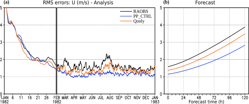
Fig. 3
The global RMS (a) analysis and (b) forecast errors (verified against the nature run) of u-winds in experiments RAOBS, PP_CTRL, and Qonly. For the analysis errors, the evolution over 1 yr is shown. Different scales on the time axis are used for the spin-up period (the first month) and the remaining 11 months. For the forecast errors, the 11-month (after the spin-up) average values are shown versus the forecast time.
RMS = root-mean-square.
Table 3
Impact of precipitation assimilation on the last 11-month averaged analysis errors of u-wind
ExperimentsGlobeNHTRSHRAOBS1.580.671.642.03PP_CTRL1.15 (−27.2%)0.53 (−20.6%)1.45 (−11.2%)0.91 (−55.2%)Qonly1.37 (−13.6%)0.58 (−13.1%)1.51 (−7.4%)1.59 (−21.8%)
[i] NH = Northern Hemisphere; SH = Southern Hemisphere; TR = tropics.
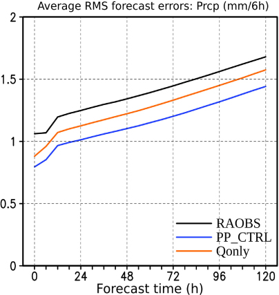
Fig. 4
As in Fig. 3b, but for precipitation forecast errors.
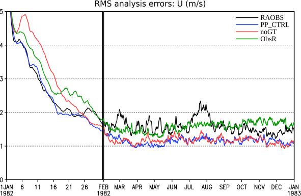
Fig. 5
As in Fig. 3a, but for experiments RAOBS, PP_CTRL, noGT, and ObsR.
Table 4
Impact of the Gaussian transformation (GT) and accuracy of precipitation observations
[i] NH = Northern Hemisphere; SH = Southern Hemisphere; TR = tropics.
Table 5
Impact of assimilation criteria of precipitation observations
ExperimentsGlobeNHTRSHRAOBS1.580.671.642.03ObsR1.58 (−0.3%)0.69 ( +3.4%)1.94 (+18.7%)1.40 (−31.0%)1mR1.29 (−18.6%)0.57 (−14.3%)1.62 (−0.9%)1.04 (−48.6%)5mR1.19 (−25.2%)0.52 (−22.3%)1.50 (−8.5%)0.94 (−53.6%)PP_CTRL (10mR)1.15 (−27.2%)0.53 (−20.6%)1.45 (−11.2%)0.91 (−55.2%)15mR1.13 (−28.9%)0.52 (−23.0%)1.42 (−13.4%)0.89 (−56.0%)
[i] NH = Northern Hemisphere; SH = Southern Hemisphere; TR = tropics.
Table 6
The average numbers and percentages (in parentheses) of observations in four classes in terms of the observation-based criterion and the model background-based criterion in PP_CTRL experiment after the spin-up
[i] Classes in bold are assimilated into the model and the others are rejected. The total number of observations is 1008 at every cycle.
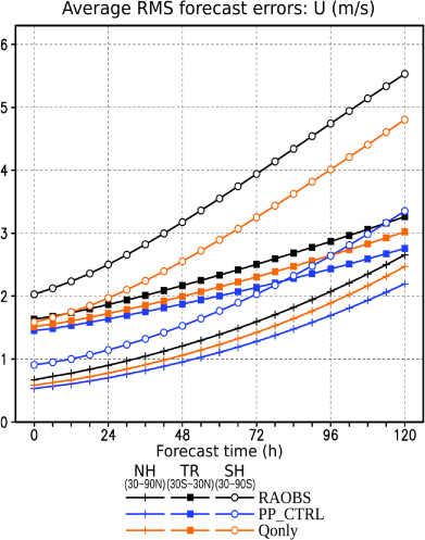
Fig. 6
As in Fig. 3b, but the RMS forecast errors are calculated separately for the NH extratropics (30–90N; NH), the tropics (30S–30N; TR), and the SH extratropics (30–90S; SH), indicated by different marks on the lines.
Table 7
Impact of horizontal localization lengths of precipitation observations
ExperimentsGlobeNHTRSHRAOBS1.580.671.642.03PP_CTRL (1L)1.15 (−27.2%)0.53 (−20.6%)1.45 (−11.2%)0.91 (−55.2%)0.5L1.07 (−32.7%)0.48 (−28.0%)1.31 (−20.0%)0.95 (−53.4%)0.3L1.14 (−27.8%)0.53 (−20.2%)1.37 (−16.2%)1.08 (−46.6%)
[i] NH=Northern Hemisphere; SH=Southern Hemisphere; TR=tropics.
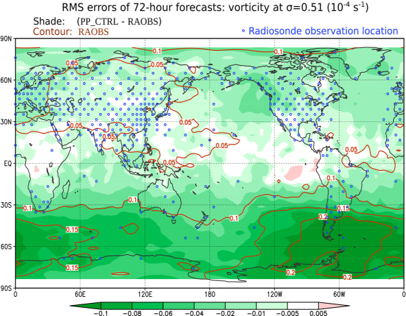
Fig. 7
The global map of RMS 72-h forecast errors of the vorticity at σ=0.51 during the 11 months after the spin-up in RAOBS (brown contour) and the corresponding error reduction from PP_CTRL to RAOBS (shading). The rawinsonde observation locations are also shown in blue open circles.
RMS=root-mean-square.
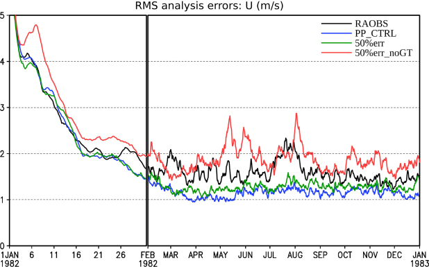
Fig. 8
As in Fig. 3a, but for experiments RAOBS, PP_CTRL, 50%err and 50%err_noGT.