
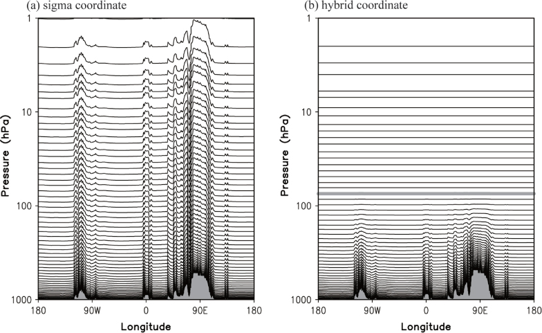
Fig. 1
Vertical profile of coordinate surface versus pressure at 34.5°N for the (a) sigma and (b) hybrid vertical coordinates at T254L64 resolution. Topographic elevations are shaded light gray. The gray contour in (b) shows the lowest-altitude isobaric level (~68 hPa).
Table 1. Summary of experiments
Table 2. A summary of test cases
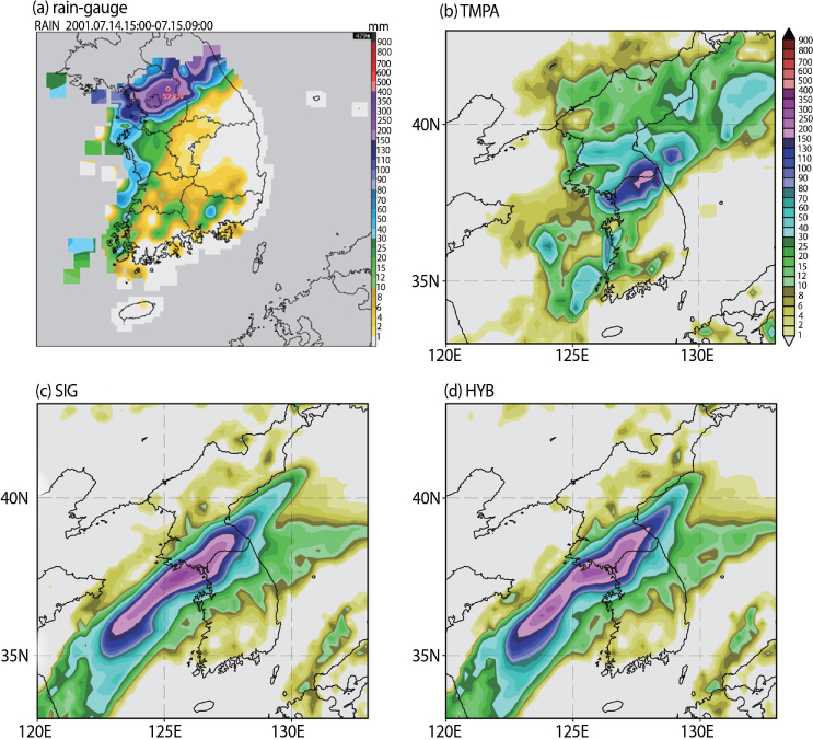
Fig. 2
Amount of 18-hour accumulated rainfall (mm) obtained from the (a) rain-gauge over South Korea and (b) TMPA data over the Korean peninsula and simulated from the (c) SIG and (d) HYB runs at T510L64 resolution.
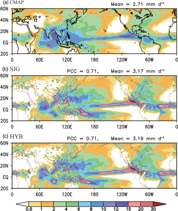
Fig. 3
June–July–August (JJA) precipitation (mm d-1) for 1996, obtained from the (a) CMAP precipitation data and simulated from the (b) SIG and (c) HYB runs at T126L28 resolution.
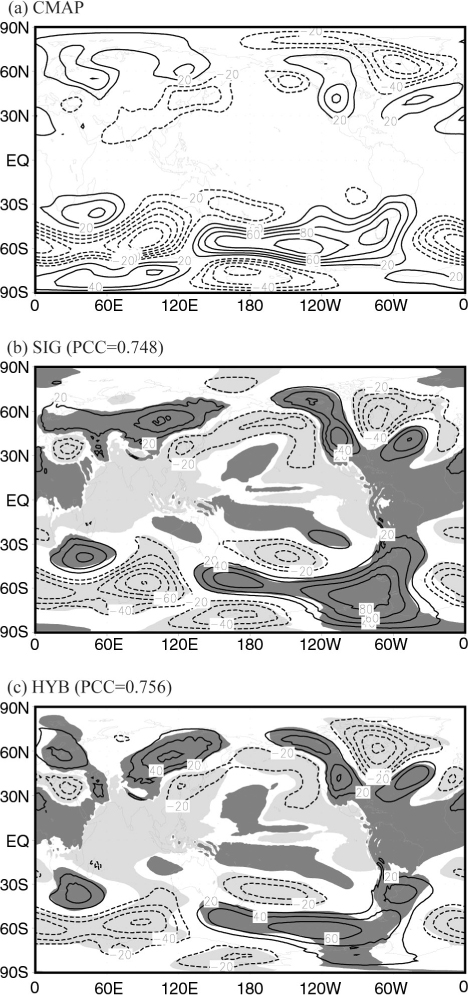
Fig. 4
Same as Fig. 3 but for 500 hPa geopotential height eddy (contour; m). Shading indicates the 95% confidence level.
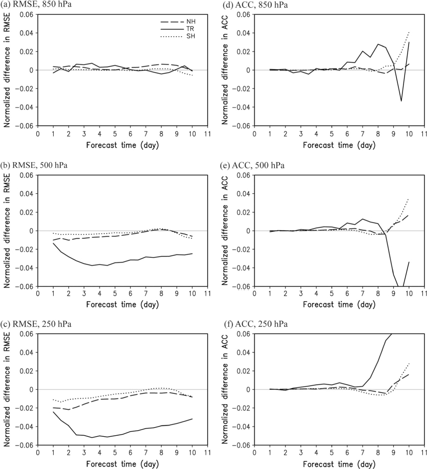
Fig. 5
Normalised difference in (left) RMSE and (right) ACC of (a),(d) 850, (b),(e) 500, and (c),(f) 250 hPa geopotential heights between the HYB and SIG runs (i.e. HYB minus SIG). The 31-ensemble members initialised at 0000 UTC are averaged at each forecast time during August 2010 and the verification is against the ERA Interim analysis in the northern hemisphere (dashed), tropics (solid), and southern hemisphere (dotted).
Table 3. Skill scores of the RMSE/anomaly correlation coefficient (ACC) for 500 hPa geopotential height (GPH) and temperature (TMP) at 5 d forecast from the SIG and HYB runs, against the ERA Interim analysis data in the northern hemisphere, tropics, and southern hemisphere. Better scores are highlighted in bold.
VariableExperiment00UTC12UTC00UTC12UTCNorthern HemisphereSIG45.5/0.81544.9/0.81861.8/0.85064.1/0.840HYB44.9/0.81744.4/0.82161.1/0.85363.6/0.842TropicsGPHSIG23.7/0.51524.2/0.52825.0/0.62825.1/0.648HYB22.2/0.51922.6/0.52623.4/0.63023.9/0.643Southern HemisphereSIG76.3/0.78575.4/0.79656.8/0.82156.9/0.817HYB76.0/0.78675.0/0.79856.7/0.82156.9/0.817Northern HemisphereSIG2.47/0.9252.45/0.9282.98/0.9563.04/0.954HYB2.43/0.9252.41/0.9282.95/0.9563.01/0.955TropicsTMPSIG2.46/0.3532.53/0.3442.01/0.5842.04/0.621HYB2.34/0.3582.41/0.3521.93/0.5881.97/0.622Southern HemisphereSIG3.30/0.9513.25/0.9532.73/0.9562.70/0.957HYB3.25/0.9523.21/0.9542.72/0.9562.68/0.957
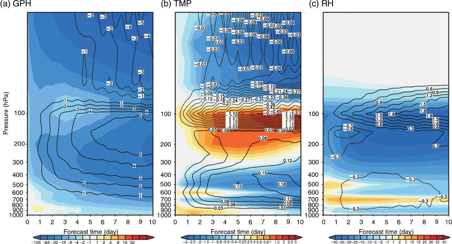
Fig. 6
Time series of the vertical profiles of the difference in (a) geopotential height, (b) temperature, and (c) relative humidity in the tropics (shading, SIG minus ERA; contour, HYB minus SIG). The 31-ensemble members initialised at 0000 UTC are averaged at each forecast time during August 2010.
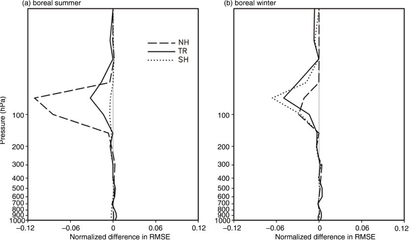
Fig. 7
Vertical profile of the normalised difference in RMSE of relative humidity between the HYB and SIG runs at forecast day 5. The 31-ensemble members initialised at 0000 UTC are averaged at each forecast time during (a) August 2010 and (b) January 2011, and the verification is against the ERA Interim analysis in the northern hemisphere (dashed), tropics (solid), and southern hemisphere (dotted).
Table 4. Same as Table 3 but simulated by the SPH dynamical core. Better scores are highlighted in bold.
VariableExperiment00UTC12UTC00UTC12UTCNorthern HemisphereSIGsph44.7/0.81643.1/0.82959.0/0.86359.1/0.864HYBsph44.7/0.81643.1/0.82958.7/0.86459.0/0.864TropicsGPHSIGsph20.7/0.54821.4/0.56422.5/0.67022.8/0.673HYBsph19.6/0.55520.2/0.56621.4/0.67121.6/0.679Southern HemisphereSIGsph73.3/0.80173.2/0.80755.6/0.82555.2/0.823HYBsph73.2/0.80172.7/0.80955.3/0.82755.0/0.824Northern HemisphereSIGsph2.38/0.9262.33/0.9312.85/0.9582.84/0.959HYBsph2.36/0.9272.31/0.9322.82/0.9592.82/0.959TropicsTMPSIGsph2.28/0.3672.34/0.3631.84/0.6121.89/0.639HYBsph2.15/0.3772.22/0.3701.76/0.6151.79/0.644Southern HemisphereSIGsph3.11/0.9553.07/0.9572.66/0.9572.60/0.959HYBsph3.09/0.9553.05/0.9572.65/0.9572.59/0.959
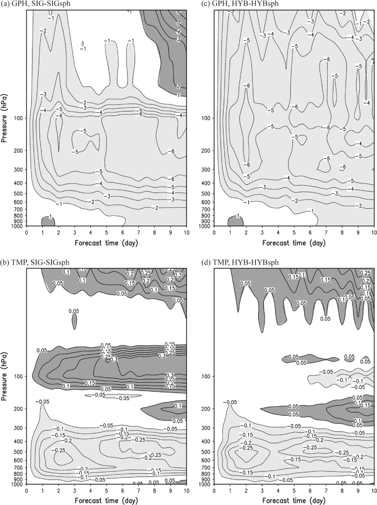
Fig. 8
Same as Fig. 6, except for the differences in (a),(c) geopotential height and (b),(d) temperature (left) between the SIG and SIGsph runs and (right) between the HYB and HYBsph runs. Contour intervals are 1 and 0.05 K for geopotential height and temperature, respectively. Heavy and light shading indicates the positive and negative bias, respectively.
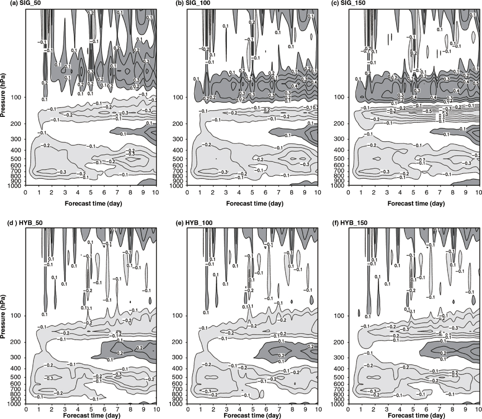
Fig. 9
Same as Fig. 8 but for temperature simulated by single-run on (a)–(c) sigma and (d)–(f) hybrid vertical coordinates. The DFS diffusion coefficient is rapidly changed at the sigma layers of (left) 0.05, (middle) 0.1, and (right) 0.15.
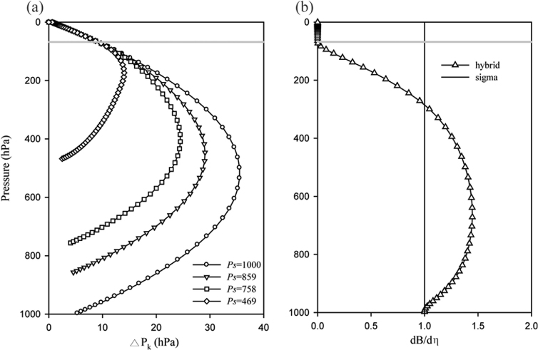
Fig. 10
(a) Layer pressure thickness versus pressure at surface pressures of 1000, 859, 758, and 469 hPa, and (b) profile of derivative of terrain-following coefficient. The gray line indicates the lowest pure pressure interface level (~68 hPa).