
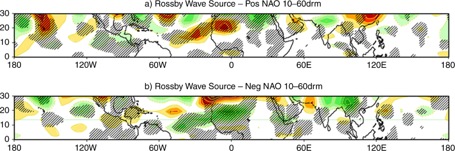
Fig. 1
Composites of RWS anomalies at 300 hPa for a) positive and b) negative NAO event days from 10–60 d means of DJF months for the period 1979–2010 using ERA–Interim data. The contour interval is 7·10−12 s −2. Negative values are shown in green. The hatched black lines indicate the areas exceeding the level of 99% significance.
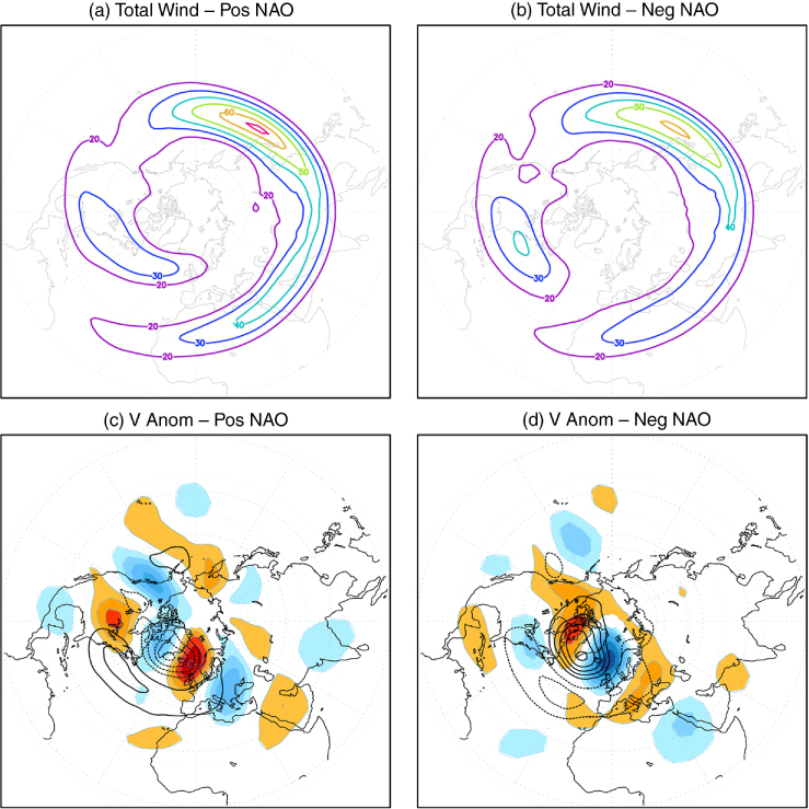
Fig. 2
Panel a) is the composite of total wind speed for positive NAO events and b) for negative events. The contour interval is 10 m/s. Composites of the meridional wind anomalies are shown in c) for positive and in d) for negative NAO events. The contour interval is 1m/s and negative values are indicated in blue colours. Over the meridional wind anomalies the geopotential height anomalies at 500 hPa are plotted. The contour interval is 35m and the negative values are indicated with dashed contours.
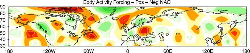
Fig. 3
Anomalies of eddy activity forcing composites of positive minus negative NAO events. The data are derived from zonal and meridional wind anomalies from ERA–Interim of DJF 1979–2010 yr. The contour interval is 6·10−12 s −2 and the green colour shades indicate negative values.
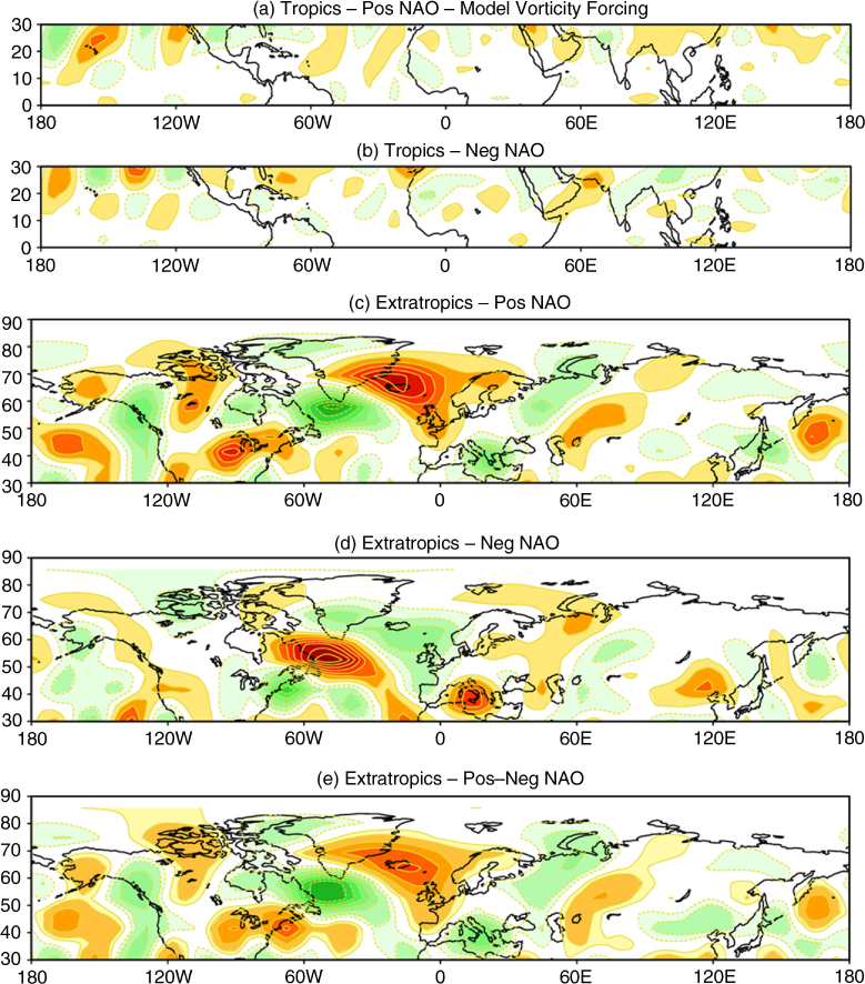
Fig. 4
Composites of anomalous vorticity forcing computed in the model by solving the BVE for a) the tropics (0°–30°N) for positive NAO events, b) for negative NAO events and for c) the extratropics (30°–90°N) for positive events and d) for negative events. At e) are the differences between positive and negative extratropical forcing. The contour interval is 4·10−12 s −2. Negative values are indicated in green.
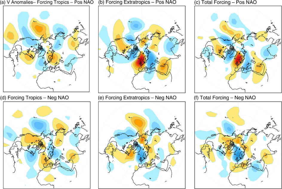
Fig. 5
Meridional wind anomalies simulated by the barotropic model when the mean circulation at 300 hPa is forced with the anomalous and run to equilibrium. First the forcing is restricted to the tropical band (0°–30°N, left panels), where in panel a) the positive NAO forcing () is used and in d) the negative NAO forcing is used (). Second, the forcing is applied only in the extratropics (30° −90°N, middle panels), similarly in b) the positive NAO forcing () is used and in e) the negative NAO forcing is used (). Finally to show the overall effect of using the anomalous NAO forcing, the entire hemisphere is forced, in c) with and in f) with . The contour intervals are 1 m/s and negative values are indicated in blue.
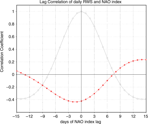
Fig. 6
Red line: a lead-lag correlation of the daily RWS index and the NAO index for DJF. The RWS index is defined as the projection of the daily RWS associated with the NAO on the total RWS composite. Grey line: an autocorrelation of the NAO index. The horizontal axis denotes the lag in days of the NAO index. The vertical axis is the correlation coefficient between lagged NAO index and RWS index, or the autocorrelation coefficient of the NAO index.
Table 1. At the left hand side the ratios of the contribution of the tropics and the extratropics for the positive and negative NAO phases are shown, quantified by the kinetic energy anomaly [eq. (8)]. At the right hand side is the zonal average of the absolute vorticity forcing , showing that the negative NAO tropical model vorticity forcing is about 14% higher in ratio between tropical–extratropical forcing than the positive phase
TropicalExtratropicalTropicalExtratropicalPos NAO14%86%1.223.4Neg NAO35%65%1.222.99
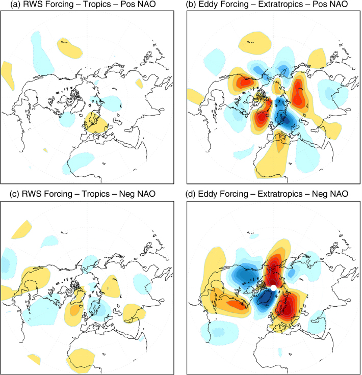
Fig. 7
Similar to Fig. 5 but instead of the model vorticity forcing, the observational forcing is applied. At a) is the response to the observed tropical RWS forcing for positive NAO events and c) for negative NAO events. In b) the forcing is the extratropical observed eddy activity for positive NAO and in d) for negative NAO. The contour intervals are 1 m/s and negative values are indicated in blue.
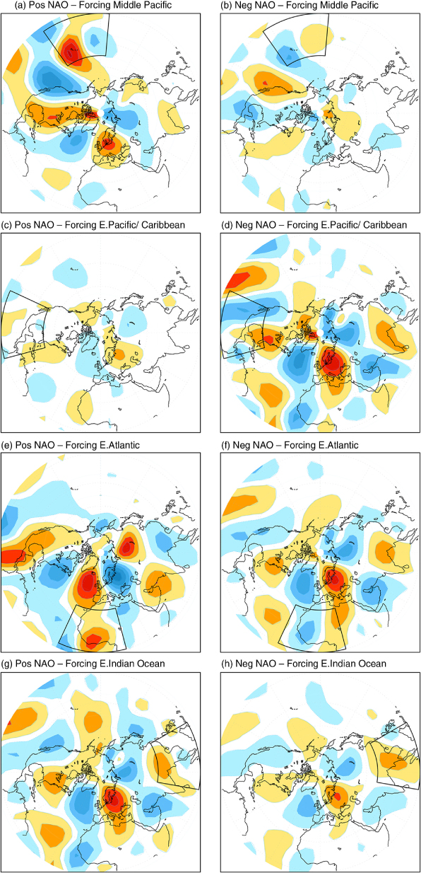
Fig. 8
Meridional wind anomalies simulated by the barotropic model when forced with the observed RWS anomalies in the tropics (0°–30°N) in constrained regions of 40°longitude. Left column for the positive NAO phase and right column for the negative phase. The forced regions are indicated by a black box. The contour intervals are 0.5 m/s and negative values are indicated in blue.