
Fig. 1.
Example BMA predictive PDF (thick curve) with the component ensemble PDFs (thin curves), the 90% confidence interval bounds (dashed vertical lines) and the verifying observation (thick solid vertical line).
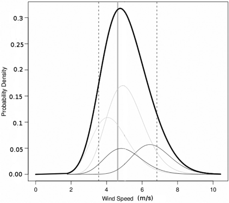
Fig. 2.
MAE, CRPS, coverage and width of 60% confidence interval for different lengths of training periods all stations. MAE, CRPS and width are negatively orientated, and lower scores are better. Coverage is considered best the closer it is to the 60% score.
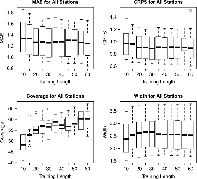
Fig. 3.
Map of the 13 forecast verification locations used in this study.
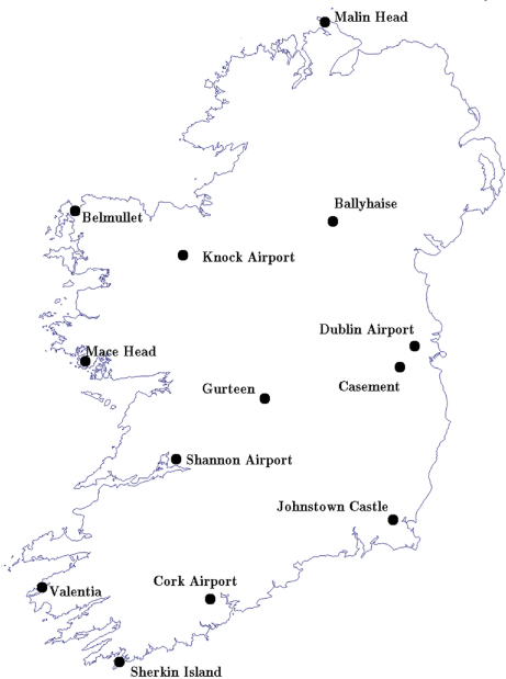
Fig. 4.
Spread-skill relationship for the daily average absolute errors in the +24 hours and +48 hours wind speed forecasts in the ECMWF EPS averaged across all stations for 1 yr. Ensemble range refers to the difference between the two ensembles at either extremes of the distribution. The correlation coefficients were +0.27 and +0.48, respectively.
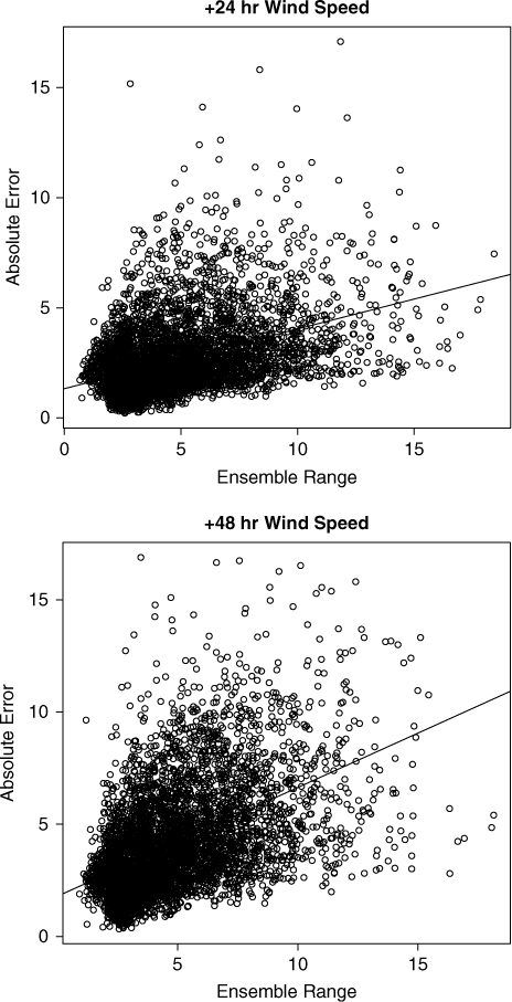
Fig. 5.
Verification rank histograms for the 51 member ECMWF EPS +24 hours and +48 hours wind speed forecasts across all stations using 12 months of data. Both VRHs show spikes at either end of the distribution indicating under-dispersion of the ensemble.
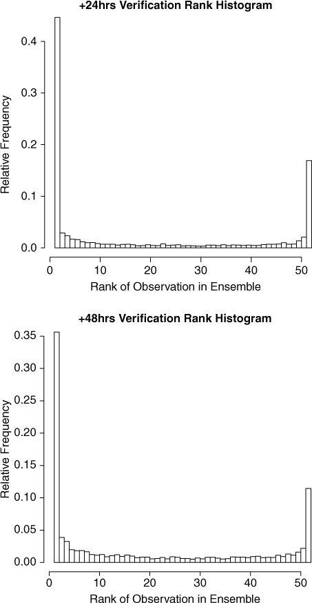
Fig. 6.
Outline of the 14 and 3 km domains used when downscaling the ECMWF representative member forecasts with COSMO and WRF.
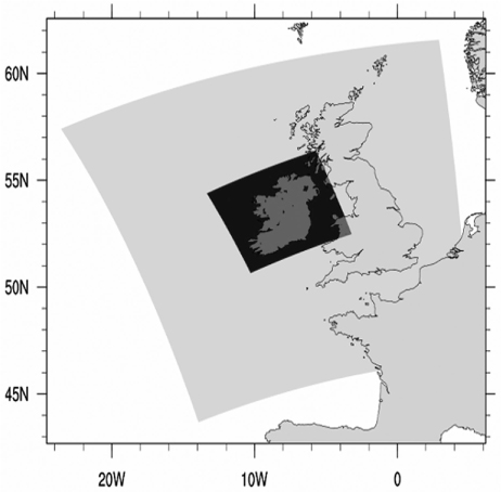
Fig. 7.
The BMA weights for the four ensemble member inputs used in Method 2 for Johnstown Castle from February 2010 to February 2011. This shows each of the members contributing significantly to the BMA forecasts at different times during the year and should all be retained for the Method 2 forecast.
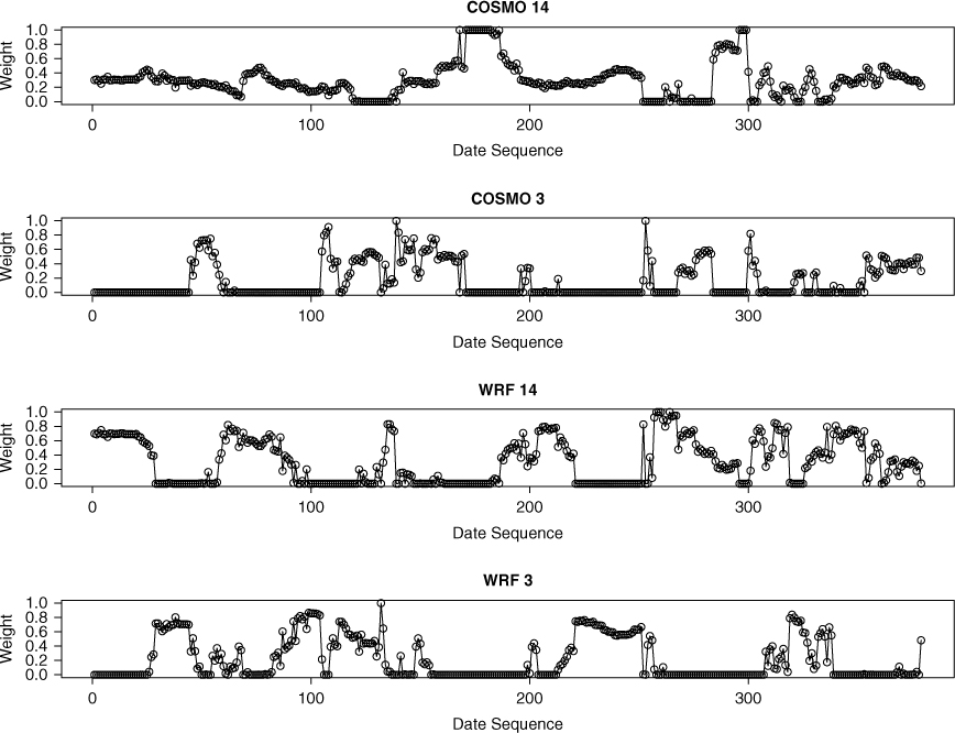
Table 1. Correlation coefficients of the forecasts errors between the four limited area model ensembles based on their weighted ensemble mean forecasts
Fig. 8.
Example VRHs for Johnstown Castle (top) and Knock Airport estimated using ECMWF EPS data. Ranks are estimated at forecast hours +24 hours for the full year of data. Johnstown Castle shows the observation falling below the ensemble range a large proportion of the time indicating an over-forecasting bias at this station. The Knock Airport histogram shows the observation falling outside the ensemble range on more occasions than within it, indicating under-dispersiveness. The dashed line corresponds to the height of the bars if the ensemble was calibrated
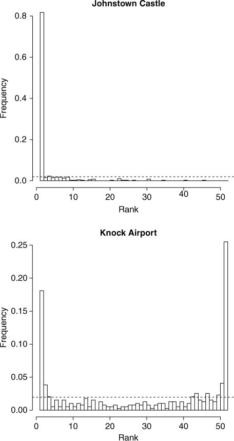
Table 2. Accuracy results for the ECMWF ensemble wind speed forecasts
[i] This table consists of the MAE, CRPS and coverage and width of the 90% prediction interval.
Fig. 9.
PIT for Johnstown Castle (top) and Knock Airport using ECMWF EPS data post-processed with BMA. The observation is compared to the full predictive PDF. The dashed line corresponds to the height of the bars if the BMA forecast was calibrated. Both PIT histograms display an over-forecasting bias but are an improvement over the uncalibrated ensemble forecast.
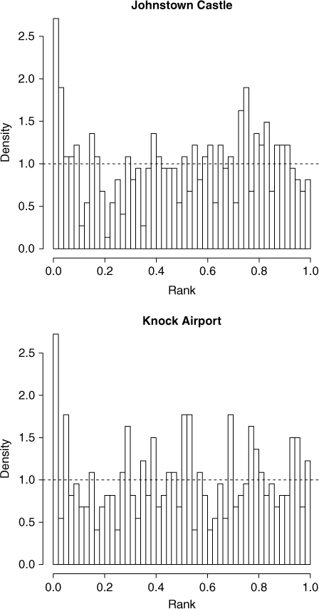
Fig. 10.
Example VRHs for a LAM forecast for Johnstown Castle (top) and Knock Airport. Ranks are estimated at forecast hours +24 hours for the full year of data. Johnstown Castle shows the observation falling below the ensemble range a large proportion of the time indicating an over-forecasting bias at this station. Knock Airport shows a similar though slightly less extreme pattern. The dashed line corresponds to the height of the bars if the ensemble was calibrated.
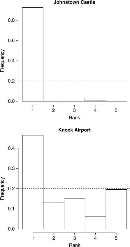
Fig. 11.
PIT for Johnstown Castle (top) and Knock Airport LAM ensemble forecasts combined and post-processed with BMA. The observation is compared to the full predictive PDF. The dashed line corresponds to the height of the bars if the BMA forecast was calibrated. Both PIT histograms show good calibration.
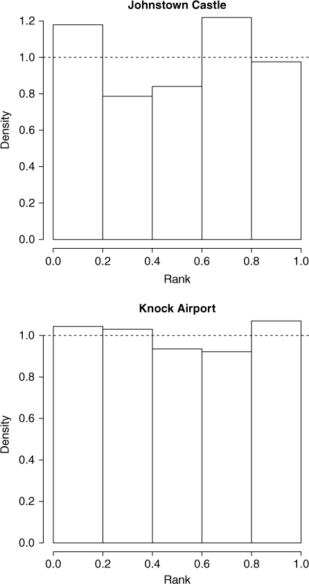
Table 3. Numerical results for ECMWF ensemble forecast and the two calibration methods for Johnstown Castle
[i] Coverage and width refer to the 90% prediction interval. The best results are displayed in bold font for clarity.
Table 4. Numerical results for ECMWF ensemble forecast and the two calibration methods for Knock Airport
[i] Coverage and width refer to the 90% prediction interval. The best results are displayed in bold font for clarity.
Table 5. Numerical results for ECMWF ensemble forecast and the two calibration methods averaged over all stations
[i] Coverage and width refer to the 90% prediction interval. The best results are displayed in bold font for clarity.